14 The singular value decomposition

14.1 Main result

Theorem 14.1 (Singular Value Decomposition) If \(A\) is an \(m \times n\) nonzero, real matrix, it can be factored as \[A = U \, \Sigma \, V^T\] where \(U\) and \(V\) are orthogonal matrices (i.e., \(U^{-1}=U^T\), \(V^{-1}=V^T\)) of dimensions \(m \times m\) and \(n \times n\), respectively, and where \(\Sigma\) is an \(m \times n \,\) ‘’diagonal matrix’’ on the form \[\begin{equation*} \Sigma = \left( \begin{array}{cccc|cccc} \sigma_1 & 0 & \ldots & \ldots & \ldots & \ldots & \cdots & 0 \\ 0 & \sigma_2 & 0 & \ldots & \ldots & \ldots & \cdots & 0 \\ \vdots & 0 & \ddots & 0 & \vdots & \vdots & \vdots & 0 \\ \vdots & \vdots & 0 & \sigma_r & 0 & \vdots & \vdots & 0 \\ \hline 0 & 0 & 0 & 0 & 0 & 0 & 0 & 0 \\ \vdots & \vdots & \vdots & \vdots & \vdots & \vdots & \vdots & \vdots \\ 0 & 0 & 0 & 0 & 0 & 0 & 0 & 0 \\ \end{array} \right) \end{equation*}\] where \(r=\text{rank}(A)\). The diagonal elements \(\sigma_{1}, \ldots, \sigma_{r}\) are called the
singular values of \(A\). These are strictly positive and ordered in such a way that The factorization \(A = U \Sigma V^T\) is called the SVD (Singular Value Decomposition) of \(A\).

Proof. Bla bla bla

14.2 Image compression based on the singular value decomposition

In this section we will analyse what kind of information the SVD captures, and illustrate how it provides a method for compressing images by reducing storage requirements.

Let \(A = U \Sigma V^T\) be the SVD of the \(m \times n\) matrix \(A\), and let \(\mathbf{u}_{j}\) and \(\mathbf{v}_{j}\) be the \(j\)-th column of \(U\) and \(V\), respectively, i.e., \[\begin{align*} U &= \begin{pmatrix} \mathbf{u}_{1} & \mathbf{u}_{2} & \cdots & \mathbf{u}_{m}\end{pmatrix} & V &= \begin{pmatrix} \mathbf{v}_{1} & \mathbf{v}_{2} & \cdots & \mathbf{v}_n\end{pmatrix}. \end{align*}\]

We start by showing that \[U \Sigma = \begin{pmatrix} \sigma_{1} \mathbf{u}_{1} & \sigma_{2}\mathbf{u}_{2} & \cdots & \sigma_{r} \mathbf{u}_{r} & \mathbf{0} & \cdots & \mathbf{0}\end{pmatrix}\] where the number of zero-vectors is \(n-r\).

Suppose first that \(1\leq j\leq r\). We then see that \((U\Sigma)_{ij} = U_{ij} \sigma_j\). Therefore we get that \(\mbox{col}_j(U\Sigma) = \sigma_j \mathbf{u}_j\). In the same way we get that \((U\Sigma)_{ij} = 0\) for \(j > r\) (since only the \(\sigma_1,...,\sigma_r\) are different from \(0\)). Therefore we get that \(\mbox{col}_j(U\Sigma) = \mathbf{0}\) for such \(j\), and the result follows.

Recall that if \(B\) is an \(m \times p\) matrix, and \(C\) is an \(p \times n\) matrix, then the matrix product \(BC\) can be written as
\[BC = \sum_{j=1}^{p}\, \texttt{col}_{j}(B) \, \texttt{row}_{j}(C).\] We use this and the above to show that \[A = \sum_{j=1}^r \, \sigma_j \, \mathbf{u}_{j}\mathbf{v}_{j}^T. \tag{14.1}\]

Since \(A=U \Sigma V^T\) we have that \[\begin{align*} A &= \sum_{j=1}^{p}\, \texttt{col}_{j}(U \Sigma) \, \texttt{row}_{j}(V^T) \\ &= \sum_{j=1}^{r} \, \sigma_j \mathbf{u}_j (\texttt{col}_{j}(V))^T = \sum_{j=1}^{r} \, \sigma_j \mathbf{u}_j \mathbf{v}_{j}^T. \end{align*}\]

Comment: The above shows that only the \(r\) first columns of \(U\) and \(V\) matter in the SVD \(A = U \Sigma V^T\). Note also that all terms in the sum Equation 14.1 are rank 1 matrices, since \(\mathbf{u}\mathbf{v}^T = [v_{1}\mathbf{u} \quad v_{2}\mathbf{u} \quad \ldots \quad v_{n}\mathbf{u}]\), so that \(\texttt{rank}( \mathbf{u}\mathbf{v}^T ) = 1\) when \(\mathbf{u}\) and \(\mathbf{v}\) are both nonzero. Thus, a matrix of rank \(r\) can be written as a sum of \(r\) rank one matrices.

14.3 Some useful Python commands

We will consider an application of the SVD to image analysis. An image can simply be considered as a matrix, a rectangular grid where each point in the grid corresponds to an element in the matrix. In image analysis one rather uses the term pixel, instead of grid point.

In gray tone images every pixel has an associated value measuring its intensity. Pixel values in such images are often stored as integers between 0 and 255, where 0 corresponds to black and 255 corresponds to white. Colour images on the other hand are often stored in the rgb-format, where every pixel has three components, one for red (r), one for green (g), and one for blue (b). All possible colours can be produced by combining these three base colours in different ways. This means that we need 3 different matrices to store an image in the rgb format. In this project we shall stick to gray tone images, so that one matrix is enough to store the image.

Below is a description of some Python commands that may be useful. \(A\) is here a two-dimensional array. We start by importing the packages we need:

import matplotlib.pyplot as plt
import numpy as np

The function in returns the rank of \(A\), and can be invoked in two ways:

r=np.linalg.matrix_rank(A)
r=np.linalg.matrix_rank(A,tol=epsilon)

The second line here requires some explanation. We are used to finding the rank by row reducing the matrix, and counting the number of pivot columns. The entries in a matrix are sensitive to roundoff errors, however. The effect of these can be that, after row reduction, it may look like the matrix has full rank, even if this is not the case. Instead we can use the fact that the rank equals the number of singular values greater than 0. Python applies this procedure, and assumes that \(\sigma_j > 0\) if \(\sigma_j > \epsilon\) for a given tolerance \(\epsilon > 0\). This tolerance is set on the second line above ().

The function in the module returns the singular value decomposition of , i.e., it returns matrices \(U\), \(V\), and a vector \(S\) so that \(A = U \Sigma V\), where \(\Sigma\) is diagonal with the entries of \(S\) on the diagonal. Note the difference from the mathematical definition in that the matrix \(V\) is not transposed!

We also have the following three functions in the module

A = np.double(plt.imread(filename,format=None))
plt.imwrite(filename,A,format=str)
plt.imshow(img,cmap='gray')

On the first line an image is read from a given file in a given format, and stored it in the matrix \(A\). Note the conversion to here, which is needed. On the second line the image stored in \(A\) is written to a given file, with the given format (to print images you have generated, use this command first, then send the resulting file to the printer). On the third line the matrix \(A\) is displayed as an image. The named parameter states that the image should be interpreted as a grayscale image (with values between 0 and 255).

We continue using the notation from above. For \(1 \leq k \leq r\) we define \[A^{(k)} = \sum_{j=1}^k \sigma_j \mathbf{u_j}\mathbf{v_j}^T. \tag{14.2}\] \(A^{(k)}\) has rank \(k\) and can thus be thought of as a rank \(k\) approximation to \(A\). How many terms we need to include, i.e., how big \(k\) must be for an acceptable approximation, will of course depend on the singular values, and how quickly they tend to \(0\).

The following function takes an \(m \times n\) matrix \(A\), and \(k\), as input, computes the SVD of the matrix, and returns the matrix \(A^{(k)}\) in Equation 14.2. If \(k > r =\text{rank}(A)\) the function provides a suitable error message:

def svdApprox(A,k):
    m,n = np.shape(A)
    assert k <= np.min([m,n]), 'we must have k<= min(m,n)!'
    U,S,V = np.linalg.svd(A)
    AK = np.zeros((m,n))
    for i in range(k):
        AK = AK + S[i]*U[:,[i]]@V[[i],:]
    return AK

The following code loads the Marilyn Monroe image mm.gif provided in this project into a matrix \(A\), checks that \(A\) is a \(256 \times 256\) matrix, and computes its rank with help of the linalg.matrix\_rank-function, and also with tolerances 0.001, 0.01, 0.1, and 1.

A = np.double(plt.imread('mm.gif'))
print(np.shape(A))
print(np.linalg.matrix_rank(A))
for k in range(-3,1):
    print(np.linalg.matrix_rank(A,tol=10**k))

The size of the matrix is printed first, followed by the different ranks.

The following code uses the function svdApprox to display the images corresponding to \(A^{(k)}\) for \(k = 8\) and \(k=32\). These are shown in Figure 14.1 and Figure 14.2

AK=svdApprox(A,8)
plt.imshow(AK,cmap='gray')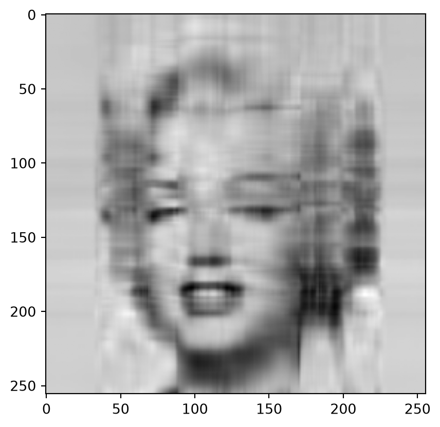

AK=svdApprox(A,32)
plt.imshow(AK,cmap='gray')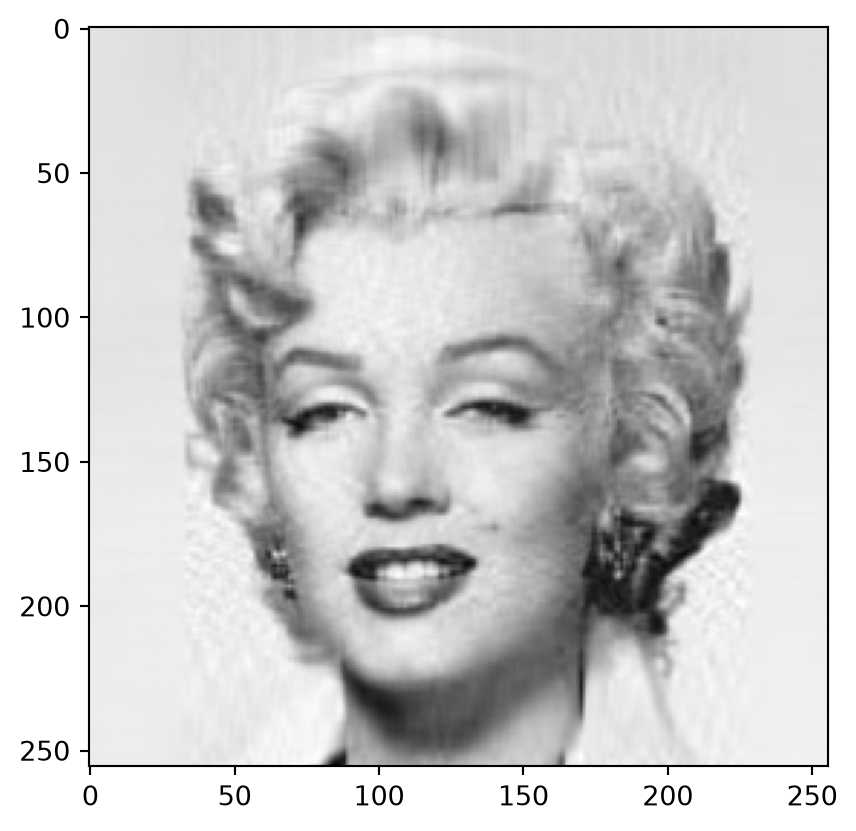

Since the rank of the image matrix equals the number of nonzero singular values, a low rank means that we can represent the matrix with just a few values. Consider the matrix below, which also is displayed as an image.

A = np.array([\
[0,32,64,96,128,160,192,224],\
[0,32,64,96,128,160,192,224],\
[0,32,64,96,128,160,192,224],\
[0,32,64,96,128,160,192,224],\
[0,32,64,96,128,160,192,224],\
[0,32,64,96,128,160,192,224],\
[0,32,64,96,128,160,192,224],\
[0,32,64,96,128,160,192,224]])
plt.imshow(A,cmap='gray')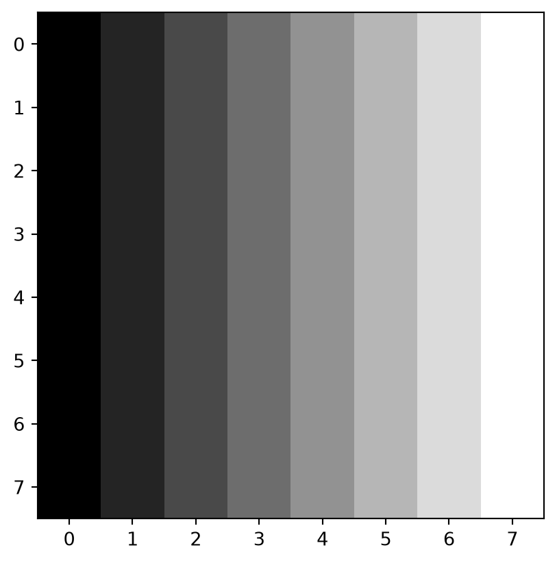

The image is constant in each column. If \(v_i\) is the value in column \(i\), the matrix can be written as \(\begin{pmatrix}1 \\ 1 \\ \vdots \\ 1\end{pmatrix}\begin{pmatrix} v_1 & v_2 & \cdots & v_n \end{pmatrix}\), which clearly is a rank one matrix.

The singular values are listed in decreasing order with the biggest first. Thus, the most ‘’important’’ information is found in the first terms in the sum in Equation 14.1.

The following code plots the singular values of the matrix corresponding to the Marilyn Monroe image (\(\sigma_j\) as a function of \(j\)). It also constructs a random image of the same size, and with pixel values in the same interval as the Marilyn Monroe image. The resulting plot is shown in Figure 14.3.

U,S1,V = np.linalg.svd(A)
plt.plot(S1)
B = (255*np.random.rand(256,256)).round()
U,S2,V = np.linalg.svd(B)
plt.plot(S2)
plt.legend(['Marilyn Monroe image','Random image'])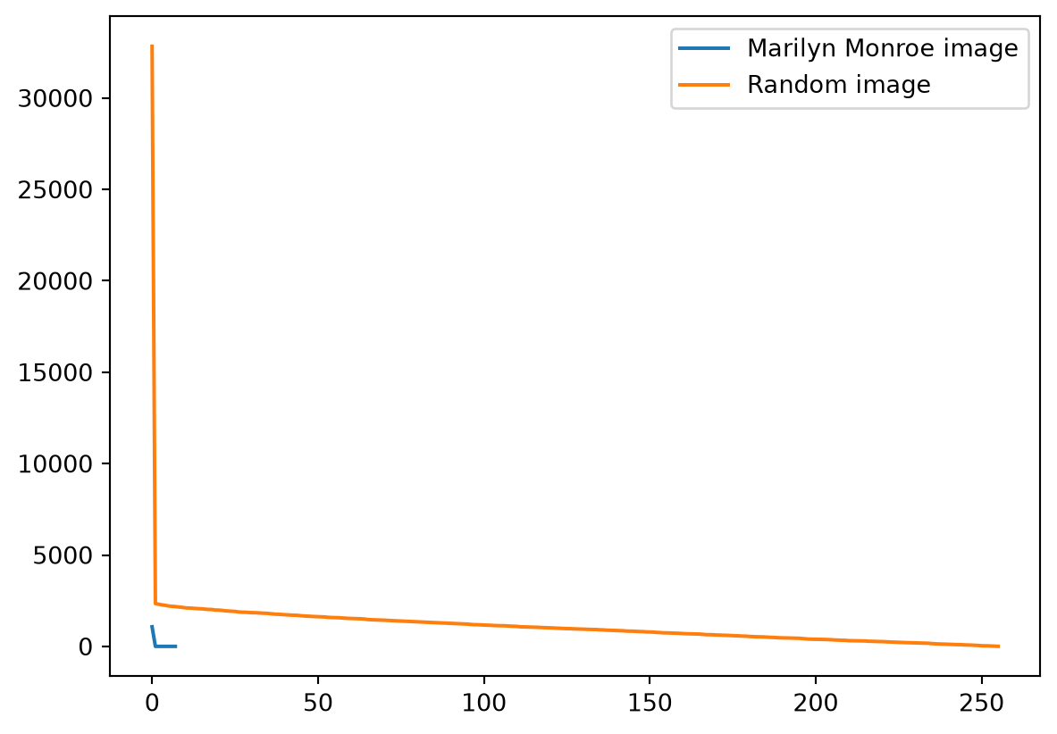

We see that the singular values decay much faster for the Marilyn Monroe image than for the random image. An informal explanation for this is that the random image has a greater degree of unorder, more ``details’’, so that one needs more singular values to describe it.

Every term in the sum Equation 14.2 needs two vectors, in addition to one singular value. To store the matrix \(A^{(k)}\) we therefore only need to store the \(k\) first vectors in both matrices \(U\) and \(V\), as well as the \(k\) first singular values. One thus needs \(k(m+n+1)\) values to store a rank \(k\) SVD approximation. This can have much to say for storage: If most of the singular values are small, we may get acceptable quality by zeroing out all singular values except the few biggest ones. As an example, a \(500\times 500\) image has 250 000 pixel values. Storing the first \(20\) singular components would require \(20\times 1001\approx 20 000\) values, which amounts to about \(8\%\) of the original storage.

As \(k\) increases the rank \(k\) SVD approximation gets visually closer to the original. For \(k\approx 50\) the quality seems to be acceptable, for \(k\approx 100\) it is near perfect.

The relative error between the matrices \(A\) and \(A^{(k)}\) is defined as \[\begin{equation*} e_{rel} = \frac{\| A - A^{(k)} \|}{ \|A\|}, \end{equation*}\] where the norm of an \(m \times n\) matrix \(B = [b_{i,j}]\) is defined by \[\| B \| = \sqrt{ \sum_{i=1}^m \sum_{j=1}^n {b_{i,j}}^2 }.\] The following function computes the relative error between the two matrices A and AK.

def relError(A,AK):
    normF = np.sqrt( np.sum((A-AK)**2) )
    normA = np.sqrt( np.sum(A**2) )
    return normF/normA

Above we reconstructed the Marylin Monroe image from the 8 first singular components, i.e., from \(A^{(8)}\). Let us now try to reconstruct the same image by using all singular values the 8 first singular components, i.e., by using the matrix \(\sum_{j=9}^r \sigma_j \mathbf{u}_{j}\mathbf{v}_{j}^T\), where \(r = \text{rank}(A)\).

The relative error when only the 8 first singular values are included is

AK1 = svdApprox(A,8)
relError(A,AK1)

np.float64(2.307936732338367e-16)

The relative error when the remaining singular values are included is

AK2 = A-AK1
relError(A,AK2)

np.float64(1.0)

The image looks as follows

plt.imshow(AK2)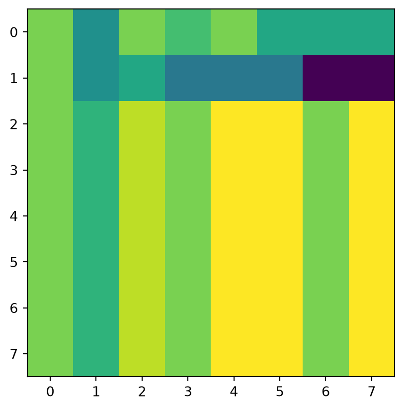

In the first image the error is about 0.1. It is far from perfect, but you can see what it is. In the other image the error is near 1 (which is the maximal we can get), and the image suffers from this.

Let \(1 \leq k \leq r\). We show that \(\{ \mathbf{u}_{1}, \, \ldots \, , \mathbf{u}_{k} \}\) is a basis for Col \(A^{(k)}\). This shows in particular that \(A^{(k)}\) has rank \(k\). This basis is orthonormal.

Note first that for \(1\leq s\leq k\) we have that \[A^{(k)}\mathbf{v}_s = \sum_{j=1}^k \sigma_j \mathbf{u_j}\mathbf{v_j}^T \mathbf{v}_s = \sigma_s \mathbf{u_s},\] since the \(\mathbf{v}_s\) provide an orthonormal basis. It follows that all \(\mathbf{u_s}\) are in the column space of \(A^{(k)}\), so that \(\texttt{Span}( \mathbf{u}_1,...,\mathbf{u}_k) \subseteq \mbox{Col}(A^{(k)})\). Since column \(s\) in \(A^{(k)}\) is \[\sum_{j=1}^k \sigma_j \mathbf{u_j}(\mathbf{v_j}^T)_s,\] it follows that also \(\mbox{Col}(A^{(k)}) \subseteq \texttt{Span}( \mathbf{u}_1,...,\mathbf{u}_k )\). Therefore \(\{ \mathbf{u}_{1}, \, \ldots \, , \mathbf{u}_{k} \}\) is a basis for \(\text{Col}(A^{(k)})\).

We have that \(A^T = V \Sigma^T U^T\), which also must be a singular value decomposition of \(A^T\). The image corresponding to \(A^T\) is not the same as the image where \(A\) is rotated 90 degrees counterclockwise: We get this if we in addition reverse the rows of \(A^T\).

\(\{ \mathbf{v}_{1}, \, \ldots \, , \mathbf{v}_{r} \}\) is a basis for Row\((A)\)= Col\((A^T)\), and this basis is orthonormal. To see this, from the above and from the singular value decomposition of til \(A^{(k)}\) it follows that \(\{ \mathbf{v}_{1}, \, \ldots \, , \mathbf{v}_{r} \}\) is a basis for Col \(A^T\), and therefore also a basis for Row \(A\).