11 Numerical differentiation

Differentiation is a basic operation in mathematics, with many applications. It is therefore important to have good methods for computing and applying derivatives. You have probably learnt the basic rules of differentiation in school - symbolic methods suitable for pen and paper calculations. These are of limited value on a computer, since many programming languages do not support symbolic computation.

Another thing is that a function may only be known in an isolated set of points, such as measurements of the position of a car with a GPS unit. Suppose we want to find the speed of the car. If the position of the car is known at all time instances (as a mathematical function), then this can be found by means of symbolic differentiation. But if the position is known for some points in time we have to appeal to other methods.

The solution is numerical methods which approximate the derivative by means of suitable combinations of known function values. Let us start by formulating this as a general algorithm: Suppose $f$ is known at the points \[...,a-2h,a-h,a,a+h,a+2h,...\] (so, $h$ is the “resolution” for known values of $f$).

Pick a subset of $n+1$ of these points near $a$, and write these as \[ a+m_0h,a+m_1h,a+m_2h,...,a+m_nh, \tag{11.1}\] where $m_0,\dots,m_n$ are integers.
Find the polynomial $p_n(x)$ interpolating $f$ in the $n+1$ points in Equation 11.1.
Use $p_n'(a)$ as an approximation to $f'(a)$.

We will also call this the point method based on the points in Equation 11.1. Point methods can be used for higher order derivatives as well, by using $p_n^{(k)}(a)$ as an approximation to $f^{(k)}(a)$. We define the truncation error in this approximation as \[ E_k(f;a,h) = f^{(k)}(a) - p_n^{(k)}(a), \] i.e., the error resulting from differentiating the interpolating polynomial rather than the function itself. The goal is to get this error as small as possible.

The simplest point methods base themselves on two known function values only, and in Section 11.1 we will see how this has a natural relation to the definition of the derivative. After this we will see how point methods with more points can produce better approximations. The methods for numerical integration in Chapter 12 will be derived and analysed the same way as the differentiation methods in this chapter.

In this chapter we will write $M_k=\max_x\left|f^{(k)}(x)\right|$ (when $f$ is $k$ times differentiable), where the maximum is taken over an interval that should be clear from the context. In the notation $p_n$ and $E_k(f;a,h)$ it should be clear from the context what the numbers $m_i$ are, even if they are not part of the notation.

11.1 The Newton quotient

The derivative of $f$ in a point $a$ is defined as \[ f'(a)=\lim_{h\rightarrow0}\frac{f(a+h)-f(a)}{h}. \tag{11.2}\] We will assume that $f$ is differentiable in $a$, i.e., this limit exists. For a fixed $h\neq 0$ the approximation \[ \frac{f(a+h)-f(a)}{h} \tag{11.3}\] to $f'(a)$ is called the Newton difference quotient, or simply the Newton quotient.

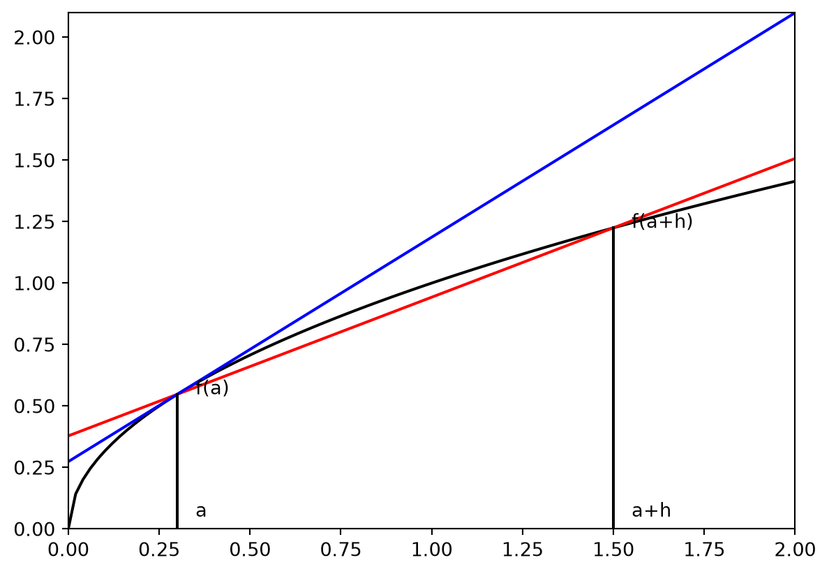
If we use the point method based on the points $a$ and $a+h$ we get the line $p_1$ through $(a,f(a))$ and $(a+h,f(a+h))$, i.e., the secant through these. This can be written \[ p_1(x)=f(a)+\frac{f(a+h)-f(a)}{h}(x-a). \] The derivative of $p_1$, i.e., the slope of the secant, is precisely the right hand side in Equation 11.3. The Newton quotient thus coincides with the point method based on $a$ and $a+h$ (see Figure 11.1).

(a) The secant (in red) of a function (in black) in the points $a$ and $a+h$, as well as the tangent in $a$ (blue).

The truncation error for the Newton quotient is \[ E_1(f;a,h) = f'(a)-\frac{f(a+h)-f(a)}{h}.\] Let us take a closer look at this. From Taylor’s formula with remainder (Equation 10.18), we get that \[ f(a+h)=f(a)+h f'(a)+\frac{h^2}{2}f''(\xi_h), \tag{11.4}\] where $\xi_h\in[a,a+h]$. Reorganising this we get the following expression for the truncation error: \[ f'(a)-\frac{f(a+h)-f(a)}{h}=-\frac{h}{2}f''(\xi_h). \tag{11.5}\] If the second derivative is continuous, the extreme value theorem says that the function $\bigl|f''\bigr|$ has a maximum on the interval $[a,a+h]$, which we denote by $M_2$. From this we get the following error estimate.

Proposition 11.1 Suppose $f$ has continuous second order derivatives near $a$. Then the truncation error of the Newton quotient satisfies \[ |E_1(f;a,h)|\le M_2\frac{h}{2}, \tag{11.6}\] where $M_2=\max_x|f''(x)|$.

When $h$ is small, $\max_{x\in [a,a+h]}|f''(x)|$ is close to $|f''(a)|$, so that the actual error is close to $|f''(a)|\frac{h}{2}$. Consider the function $f(x)=\sin x$ at the point $a=0.5$. We have $f''(x)=-\sin (x)$, so that for small $h$ the error in the Newton quotient is about $\frac{\sin 0.5}{2}h\approx 0.24h$.

It is common also to the worse bound $M_2=\max_{x\in\mathbb{R}}|f''(x)|=1$, rather than $\max_{x\in [a,a+h]}|f''(x)|$. This gives the bound $|E_1(f;a,h)| \leq 0.5 h$ for the Newton quotient, which is an overestimate of the error with a factor of about $2$. In error estimates it is common to miss a bit, and “exaggerate” how large the error can become. The central point here is that we have estimated something unknown (the error $E_1$) with something computable (the right hand side in Equation 11.6).

The error $e$ in our numerical methods will usually be on the form $e=Kh^k$, where $h$ is the precision in the method, and the constant $K$ and the exponent $k$ are unknown. We then say that $y$ is polynomial in $x$, with constant $K$ and exponent $k$. A loglog plot can help us find out if there are such relations between $h$ and $e$, and if so help us estimate the concrete values of $K$ and $k$. If we plot $h$ against $e$ it is not so easy to grasp $K$ and $k$ from the plot, since the curves ascend quickly. A trick can then be to take logarithms, which gives \[ \log e = \log K + k\log h.\] In other words, if we plot the logarithm of the error against the logarithm of $h$, we obtain a line where

the slope of the curve gives us the exponent $k$, and
the intersection with the $y$-axis is in $\log K$, so that we can find $K$ from this intersection.

We write plt.loglog(h,e) to plot $\log h$ against $\log e$. plt.loglog has a syntax similar to that of the plt.plot-command.

Figure 11.2 shows a loglog plot of $h$ against the truncation error, together with the upper bound $M_2h/2$ for the error. Here we set $M_2=1$, so that we again produce an overestimate. A better estimate could be obtained by finding $\max_x|f''(x)|$ over a small interval near $a$ instead, but if you do this you will see that the two curves lie on top of one-another.

f = np.sin
fd = np.cos
a = 0.5
h = 10**(-np.arange(0,6,0.1).reshape(-1,1))
efh = fd(a) - (f(a+h)-f(a))/h
plt.loglog(h, np.abs(efh), 'k.', h, h/2, 'r')
plt.legend(['Error','Bound on error'])

Figure 11.2: The truncation error of the Newton quotient when $f(x)=\sin x$ at the point $x=0.5$, for $h\in [10^{-6},10^0]$. The plot is logarithmic.

The plot looks like a line with slope $1$. Since the plot is logarithmic, this agrees with the approximation $|E_1(f;a,h)|\approx\frac{h}{2}|f''(a)|$ for the truncation error, since we obtain by taking logarithms in this that \[\begin{align*} \log |E_1(f;a,h)|&\approx\log h + \log(0.5) + \log(\sin(0.5)) \\ &\approx \log h - 0.6203. \end{align*}\] This agrees well with the point where the line hits the $y$-axis. $\clubsuit$

11.2 The symmetric Newton quotient

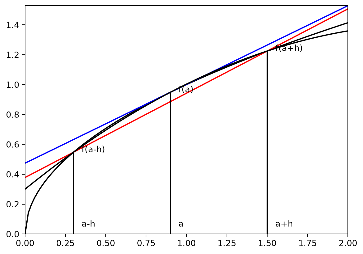
The Newton quotient was based on the points $f(a)$ and $f(a+h)$. Let us instead consider the points $f(a)$, $f(a-h)$, and $f(a+h)$. Using the Newton form of the interpolating polynomial we get from Equation 10.13 and Equation 10.14 that \[ \begin{aligned} p_2(x) =&\, f(a-h) + \frac{f(a)-f(a-h)}{h}(x-(a-h)) \\ &+ \frac{f(a+h)-2f(a)+f(a-h)}{2h^2}(x-(a-h))(x-a). \end{aligned} \tag{11.7}\] After some computation we get \[ p_2'(a)=\frac{f(a+h)-f(a-h)}{2h} \tag{11.8}\] We leave the details in Equation 11.7 and Equation 11.8 to Exercise 11.4. Equation 11.8 gives the slope of the secant through the points $a-h$ and $a+h$, and is called the symmetric Newton quotient. This is illustrated in Figure 11.3,

(a) The secant based on $a-h$ and $a+h$ (in red) of a function $f$ (in black), as well as the tangent in $a$ (in blue). The parabola interpolating $f$ in $a-h$, $a$, and $a+h$ are also shown (in black)

The truncation error of the symmetric Newton quotient can be analysed in the same way as the Newton quotient. We now evaluate the Taylor polynomial at two points, and include a quadratic term instead: \[\begin{align*} f(a+h) &= f(a) + f'(a)h + \frac{1}{2}f''(a)h^2 + \frac{1}{6}f'''(c_1)h^3\\ f(a-h) &= f(a) - f'(a)h + \frac{1}{2}f''(a)h^2 - \frac{1}{6}f'''(c_2)h^3, \end{align*}\] where $c_1\in[a,a+h]$, $c_2\in[a-h,a]$. Subtracting these we get \[\frac{f(a+h)-f(a-h)}{2h}-f'(a)=\frac{1}{12}h^2(f'''(c_1)+f'''(c_2)).\] If we take the absolute value of both sides and use the triangle inequality we get that \[|E_1(f;a,h)| = \left| \frac{1}{12}h^2(f'''(c_1)+f'''(c_2)) \right| \leq \frac{h^2}{12}M_3 + \frac{h^2}{12}M_3 = M_3\frac{h^2}{6}.\] The approximation will in particular be exact for quadratic polynomials, since these have a third derivative equal to 0 (so that $M_3=0$). The truncation error is therefore 0 for these. The approximation is not exact for cubic polynomials.

11.3 A point method for the second derivative

To derive a point method for the second derivative, we will use the same points as for the symmetric Newton quotient, This gives the same interpolating polynomial as in Equation 11.7. After some computation we find that \[ p_2''(a)=\frac{f(a+h)-2f(a)+f(a-h)}{h^2} \tag{11.9}\] As above we can find the truncation error by evaluating the Taylor polynomial in the same points, but we now also include a cubic term, \[\begin{align*} f(a+h) &= f(a) + f'(a)h + \frac{1}{2}f''(a)h^2 + \frac{1}{6}f'''(a)h^3 + \frac{1}{24}f^{(iv)}(c_1)h^4\\ f(a-h) &= f(a) - f'(a)h + \frac{1}{2}f''(a)h^2 - \frac{1}{6}f'''(a)h^3 + \frac{1}{24}f^{(iv)}(c_2)h^4, \end{align*}\] and instead of subtracting the two we now add them together. We then get \[ f(a-h)-2f(a) + f(a+h) - f''(a)h^2 = \frac{1}{24}f^{(iv)}(c_1)h^4 + \frac{1}{24}f^{(iv)}(c_2)h^4. \] Dividing with $h^2$ on both sides we get the truncation error \[|E_2f(;a,h)| = \left| \frac{f(a-h)-2f(a) + f(a+h)}{h^2} - f''(a) \right|\] on the left side, and on the right side we get \[M_4\frac{h^2}{24} + M_4\frac{h^2}{24} = M_4\frac{h^2}{12}.\]

11.4 More general point methods

For point methods with more points one can also do as above - i.e., combining Taylor series evaluated in the known points so that one on the left side gets an expression for the truncation error. We need the following result, which uses linear algebra to derive the general point method based on $f(a+m_0h)$, $f(a+m_1h),\dots,f(a+m_nh)$.

Theorem 11.1 Suppose we know $n+1$ function values $\{f(a+m_ih)\}_{i=0}^n$, where $m_0=0$ and $m_0,m_1,\dots,m_n$ are distinct integers (we assume in particular that $f(a)$ should contribute). Let $p_n$ be the interpolating polynomial of $f$ of degree $\leq n$ in the points $\{a+m_ih\}_{i=0}^n$. Then we have that \[ \begin{pmatrix} h^1p_n^{(1)}(a)/1! \\ h^2p_n^{(2)}(a)/2! \\ \vdots \\ h^np_n^{(n)}(a)/n! \end{pmatrix} = \begin{pmatrix} m_1 & m_1^2 & \cdots & m_1^n \\ m_2 & m_2^2 & \cdots & m_2^n \\ \vdots & \vdots & \ddots & \vdots\\ m_n & m_n^2 & \cdots & m_n^n \end{pmatrix}^{-1} \begin{pmatrix} f(a+m_1h) - f(a) \\ f(a+m_2h) - f(a) \\ \vdots \\ f(a+m_nh) - f(a) \end{pmatrix}. \tag{11.10}\]

You are not supposed to remember this result! The point is that we from this actually can read out, and write code to code to find the approximations $p_n^{(k)}(a)$ to all the derivatives! We obtain the approximations by solving a system involving a Vandermonde matrix.

Proof. $p_n$ equals its own Taylor series of degree $\leq n$ om $a$, i.e., that \[p_n(x) = p_n(a)+p_n'(a) (x-a)+\cdots + \frac{p_n^{(n)}(a)}{n!}(x-a)^n.\] Evaluating this in $x=a+m_ih$ we get that \[f(a+m_ih) = f(a)+p_n'(a) m_ih+\cdots + \frac{p_n^{(n)}(a)}{n!}m_i^nh^n,\] which can be written \[ f(a+m_ih) - f(a) = \begin{pmatrix} m_i & m_i^2 & \cdots & m_i^n \end{pmatrix} \begin{pmatrix} hp_n'(a) \\ h^2p_n^{(2)}(a)/2! \\ \vdots \\ h^np_n^{(n)}(a)/n! \end{pmatrix} \] for $i=1,2,\dots,n$ qw assemble this to \[\begin{align*} \begin{pmatrix} m_1 & m_1^2 & \cdots & m_1^n \\ m_2 & m_2^2 & \cdots & m_2^n \\ \vdots & \vdots & \ddots & \vdots \\ m_n & m_nh^2 & \cdots & m_n^n \end{pmatrix} \begin{pmatrix} h^1p_n^{(1)}(a)/1! \\ h^2p_n^{(2)}(a)/2! \\ \vdots \\ h^np_n^{(n)}(a)/n! \end{pmatrix} = \begin{pmatrix} f(a+m_1h) - f(a) \\ f(a+m_2h) - f(a) \\ \vdots \\ f(a+m_nh)-f(a) \end{pmatrix}, \end{align*}\] The matrix on the left side is an invertible Vandermonde matrix. Multiplying with its inverse on both sides gives the needed expression.

Let us consider some examples.

Example 11.1 Let us consider point methods based on the three points $a$, $a-h$, and $a+h$. This corresponds to setting $n=2$, $m_1=-1$, $m_2=1$. Equation 11.10 gives \[\begin{align*} \begin{pmatrix}hp_2'(a) \\ h^2p_2''(a)/2\end{pmatrix} &= \begin{pmatrix} m_1 & m_1^2 \\ m_2 & m_2^2 \end{pmatrix}^{-1} \begin{pmatrix} f(a-h)-f(a) \\ f(a+h)-f(a)\end{pmatrix} = \begin{pmatrix}-1 & 1 \\ 1 & 1\end{pmatrix}^{-1} \begin{pmatrix} f(a-h)-f(a) \\ f(a+h)-f(a)\end{pmatrix} \\ &= \frac{1}{2}\begin{pmatrix} -1 & 1 \\ 1 & 1\end{pmatrix} \begin{pmatrix} f(a-h)-f(a) \\ f(a+h)-f(a)\end{pmatrix} = \begin{pmatrix} \frac{f(a+h)-f(a-h)}{2} \\ \frac{f(a-h)-2f(a)+f(a+h)}{2} \end{pmatrix}. \end{align*}\] This can be rewritten to \[\begin{align*} p_2'(a) &= \frac{f(a+h)-f(a-h)}{2h} \\ p_2''(a) &= \frac{f(a-h)-2f(a)+f(a+h)}{h^2}\end{align*}\] We see that this coincides with the point methods from Equation 11.8 and Equation 11.9. $\clubsuit$

Example 11.2 Let us consider point methods based on the five points $a$, $a-2h$, $a-h$, $a+h$, and $a+2h$. We set $n=4$, $m_1=-2$, $m_2=-1$, $m_3=1$, $m_4=2$. Equation 11.10 gives \[\begin{align*} \begin{pmatrix} h^1p_4^{(1)}(a)/1! \\ h^2p_4^{(2)}(a)/2! \\ h^3p_4^{(3)}(a)/3! \\ h^4p_4^{(4)}(a)/4! \end{pmatrix} &= \begin{pmatrix} m_1 & m_1^2 & m_1^3 & m_1^4 \\ m_2 & m_2^2 & m_2^3 & m_2^4 \\ m_3 & m_3^2 & m_3^3 & m_3^4 \\ m_4 & m_4^2 & m_4^3& m_4^4 \end{pmatrix}^{-1} \begin{pmatrix} f(a-2h) - f(a) \\ f(a-h) - f(a) \\ f(a+h)-f(a) \\ f(a+2h)-f(a)\end{pmatrix} \\ &= \begin{pmatrix} -2 & 4 & -8 & 16 \\ -1 & 1 & -1 & 1 \\ 1 & 1 & 1 & 1 \\ 2 & 4 & 8 & 16 \end{pmatrix}^{-1} \begin{pmatrix} f(a-2h) - f(a) \\ f(a-h) - f(a) \\ f(a+h)-f(a) \\ f(a+2h)-f(a)\end{pmatrix} \end{align*}\] It is smart to find the inverse matrix symbolically here:

V = sym.Matrix([[-2,4,-8,16],[-1,1,-1,1],[1,1,1,1],[2,4,8,16]])
V.inv()

$\displaystyle \left[\begin{matrix}\frac{1}{12} & - \frac{2}{3} & \frac{2}{3} & - \frac{1}{12}\\- \frac{1}{24} & \frac{2}{3} & \frac{2}{3} & - \frac{1}{24}\\- \frac{1}{12} & \frac{1}{6} & - \frac{1}{6} & \frac{1}{12}\\\frac{1}{24} & - \frac{1}{6} & - \frac{1}{6} & \frac{1}{24}\end{matrix}\right]$

The expression above therefore becomes \[\begin{align*} \begin{pmatrix} 1/12 & -2/3 & 2/3 & -1/12 \\ -1/24 & 2/3 & 2/3 & -1/24 \\ -1/12 & 1/6 & -1/6 & 1/12 \\ 1/24 & -1/6 & -1/6 & 1/24 \end{pmatrix} \begin{pmatrix} f(a-2h) - f(a) \\ f(a-h) - f(a) \\ f(a+h)-f(a) \\ f(a+2h)-f(a)\end{pmatrix} \end{align*}\] Evaluating the first row we get \[\begin{align*} hp_4'(a) &= \begin{pmatrix}1/12 & -2/3 & 2/3 & -1/12 \end{pmatrix} \begin{pmatrix} f(a-2h) - f(a) \\ f(a-h) - f(a) \\ f(a+h)-f(a) \\ f(a+2h)-f(a)\end{pmatrix} \\ &= \frac{f(a-2h)}{12} - \frac{2f(a-h)}{3} + \frac{2f(a+h)}{3} - \frac{f(a+2h)}{12} - \left( \frac{1}{12} - \frac{2}{3} + \frac{2}{3} - \frac{1}{12}\right)f(a) \\ &= \frac{f(a-2h) -8f(a-h) +8f(a+h)-f(a+2h)}{12}. \end{align*}\] Dividing by $h$ we get \[p_4'(a) = \frac{f(a-2h) -8f(a-h) +8f(a+h)-f(a+2h)}{12h}.\]

11.5 Summary

Let us return to the function $f(x)=\sin (x)$, at the point $a=0.5$. Since the derivative is $f'(x)=\cos (x)$, and $f'(a)\approx0.8775825619$, it is easy to check the accuracy in the methods we have derived. The errors with $h=10^{-1},10^{-2},...,10^{-6}$ for three of the methods are shown in Table 11.1.

Table 11.1: Truncation errors for different $h$ for the three methods we have considered.

h	Newton	Symmetric Newton	Four point method
0.100000	2.541321e-02	1.461906e-03	2.921795e-06
0.010000	2.411734e-03	1.462630e-05	2.925231e-10
0.001000	2.398590e-04	1.462637e-07	5.773160e-15
0.000100	2.397274e-05	1.462736e-09	7.516210e-14
0.000010	2.397147e-06	1.750344e-11	5.476064e-12
0.000001	2.396897e-07	7.476686e-12	7.476686e-12

Each time $h$ is divided by 10 we see that

for the Newton quotient, the truncation error is reduced by a factor of about $10$. This is as expected since the truncation error was shown to be $M_2\frac{h}{2}$.
for the symmetric Newton quotient, the error gets reduced by a factor of about 100. This is as also expected since the truncation error was shown to be $M_3\frac{h^2}{6}$.
for the four point method, the error gets reduced by a factor of about 10000. This follows from that the truncation error satisfies $|E_1(f;a,h)|\leq\frac{M_5}{18}h^4$, which we state without proof.

Let us also make loglog plots of the truncation errors. For this we will also include the second derivative, which had a truncation error bounded by $M_4\frac{h^2}{12}$. We will also use that $M_k\approx (\sin a)^{(k)}$ near $a$. The truncation error bounds are plotted against each other as follows.

a=0.5
h = 10**(-np.arange(0,6,0.1))
plt.loglog(h, np.abs(np.sin(a)*h/2),
               h, np.abs(np.cos(a)*h**2/6),
               h, np.abs(18*np.cos(a)*h**4),
               h, np.abs(np.sin(a)*h**2/12))
plt.legend(['Newton','Symmetric Newton',
            'Four points','second derivative'])

Figure 11.4: loglog plot of the estimates of the truncation errors for the four methods we have considered, for $f(x)=\sin x$ in $x=0.5$, and for $h\in [10^{-6},10^0]$.

Note that, if $|E_1(f;a,h)|\approx Ch^p$, we have that \[\log|E_1(f;a,h)|\approx p\log h+\log C.\] Our methods have truncation errors proportional to $h$, $h^2$, and $h^4$. This is why we see lines with slopes $1$, $2$, and $4$ in the loglog plot.

Quiz

--- primary_color: orange secondary_color: lightgray text_color: black shuffle_questions: false shuffle_answers: false --- ## Method for approximating the second derivative We approximate the second derivative of a function $f(x)$ in $x=0$ with $$ D_2 f(0) = \frac{f(h) - 2f(0) + f(-h)}{h^2} $$ We assume that $f$ is differentiable an infinite number of times. The approximation $D_2 f(0)$ will always be exact if $f(x)$ is > The approximation is exact for all polynomials of degree 3 since $M_4=0$ for these (the fourth derivative of a cubic polynomial is 0). If we try with $f(x)=x^4$ the approximation is $\frac{h^4+h^4}{h^2}=h^2$, which is different from $f''(0)=0$. 1. [ ] a trigonometric function 2. [ ] a logarithmic function 3. [ ] a polynomial of degree 4 4. [x] a polynomial of degree 3 ## Error in the method for approximating the second derivative. The error $\left| f^{\prime\prime} (0) - D_2f(0) \right|$ is limited by 1. [ ] $\frac{h^2}{12}\max_{x\in[-h,h]}\left| f^{\prime\prime}(x)\right|$ 2. [ ] $\frac{h^2}{48}\max_{x\in[-h,h]}\left| f^{(4)}(x)\right|$ 3. [ ] $\frac{h}{4}\max_{x\in[-h,h]}\left| f^{\prime\prime}(x)\right|$ 4. [ ] $\frac{h^2}{12}\max_{x\in[-h,h]}\left| f^{(4)}(x)\right|$ ## The symmetric Newton quotient The symmetric Newton quotient is exact for polynomials of degree 2 or lower. > Since $M_3=0$ for all quadratic polynomials, and since the symmetric Newton quotient has truncation error $\leq M_3\frac{h^2}{6}$, then the symmetric Newton quotient is exact for all quadratic polynomials. 1. [x] True 2. [ ] False ## Comparison of Symmetric Newton and Newton. Even if the symmetric Newton quotient has higher precision than the Newton quotient, there is a trade-off since it requires much more computation than the Newton quotient. 1. [ ] True 2. [x] False ## Comparison of Newton and the four point method The four point method with step length $h=0.2$ will usually have less error than the Newton quotient with $h=0.1$. > The four point method has error proportional to $h^4$, and $0.2^4$ is much smaller than $0.1$. 1. [x] True 2. [ ] False ## Exactness of the four point method The four point method is exact for all fourth degree polynomials, but not for all fifth degree polynomials. > Since $M_5=0$ for all fourth degree polynomials, and since the four point method has truncation error $\leq \frac{M_5}{18}h^4$, the four point method is exact for all fourth degree polynomials. If we try with $f(x)=x^5$ the approximation to the derivative in $0$ is $$ \frac{(-2h)^5 -8(-h)^5+8h^5-(2h)^5}{12h} = \frac{h^5(-32+8+8-32)}{12h} = -4h^4, $$ while $f'(0)=0$, so that the method is not exact for $f(x)=x^5$. 1. [x] True 2. [ ] False

Exercises

Exercise 11.1 (Left sided Newton quotient) An alternative to the Newton quotient in Equation 11.3 is the left sided variant \[ f'(a)\approx \frac{f(a)-f(a-h)}{h}. \] Show that this coincides with the point method based on $a$ and $a-h$.

Exercise 11.2 Write a program which computes the Newton quotient for the function $f(x)=e^x$ in $a=1$, and uses $h=10^{-k}$ for $k=1$, $2$, , $14$. Also compute the error. Does the approximation and its error behave as Proposition 11.1 predicts?

Exercise 11.3 When deriving the truncation error in Equation 11.6, it was not obvious what the degree of the Taylor polynomial in Equation 11.4 should be. In this exercise you will see what happens when one decreases the degree of the Taylor polynomial.

Redo the Taylor expansion in Equation 11.4 again, but this time use a Taylor polynomial of degree $2$. Try from this to derive a formula for the error corresponding to Equation 11.5.

Repeat (a), but use a Taylor series of degree $0$, i.e., a constant.

Why can you conclude that the first order Taylor polynomial and the formula for the error in Equation 11.5 is best?

Exercise 11.4 Show that Equation 11.7 Equation 11.8 are correct.

Exercise 11.5 Show that the symmetric Newton quotient in $x=a$

equals $f'(a)$ when $f$ is a quadratic polynomial $f(x)=bx^2+cx+d$.

equals the average of the two asymmetric quotients \[\begin{aligned} f_{r}(a)&=\frac{f(a+h)-f(a)}{h} & f_{l}(a)&=\frac{f(a)-f(a-h)}{h}.\end{aligned} \tag{11.11}\]

Exercise 11.6 In this exercise we consider some other possible approximations to the derivative.

Find an approximation to $f'(a)$ which only uses the values $f(a-h)$, $f(a)$, and $f(a+2h)$.

Find an approximation to $f'(a)$ which only uses the values $f(a)$, $f(a+h)$, and $f(a+2h)$.

Exercise 11.7 This exercise illustrates another method way to derive methods for numerical differentiation.

Suppose we want to derive a method for approximating $f'(a)$ on the form \[ f'(a)\approx c_1 f(a-h)+ c_2 f(a+h), \quad c_1, c_2\in\mathbb{R}. \] We want the method to be exact when $f(x)=1$ and $f(x)=x$. Use these requirements to compute $c_1$ and $c_2$.

Show that the method in (a) is exact for all polynomials of degree one, and compare it with the methods we have derived in this chapter.

Use the methods in (a) and (b) to derive a method for approximating $f''(a)$, \[ f''(a)\approx c_1 f(a-h)+c_2 f(a)+c_3 f(a+h), \quad c_1, c_2, c_3\in \mathbb{R}, \] demanding that the method should be exact for $f(x)=1$, $x$, and $x^2$. Do you recognise this method?

Show that the method in (c) is exact for all cubic polynomials.

Exercise 11.8 In this exercise we will compare the symmetric Newton quotient with the two asymmetric Newton quotients.

Plot the graph of the function \[ f(x)=\frac{-x^{2}+10x-5}{4} \] over the interval $[0,6]$, together with the three secants corresponding to the three approximations to the derivative from (a) (use $a=3$ and $h=2$). Can you from this decide which approximation is best?

Compute the three approximations to the derivatives in (a) numerically for $f(x)$ with $a=3$ and $h_{1}=0.1$ and $h_{2}=0.001$. What are the relative errors?