def plot_regression(x, f, nvals):
    for n in nvals:
        p = np.arange(0,n+1).reshape((1,-1))
        A = x**p
        sol = np.linalg.solve(A.T@A,A.T@f)
        t = np.linspace(0,3.5,100).reshape((-1,1))
        plt.plot( t, t**p@sol, label = f"n={n}" )
    plt.scatter(x,f)
plt.legend()13 Orthogonality and least squares
13.1 Orthogonal decomposition theorem
The following generalises Proposition 1.4.
Proposition 13.1 (Orthogonal decomposition theorem, general version) Let \(\mathcal{B}\) be a subspace of \(\mathbb{R}^n\). Any \(\mathbf{a}\in\mathbb{R}^n\) can be written uniquely as \(\mathbf{p}+(\mathbf{a}-\mathbf{p})\) with \(\mathbf{p}\in\mathcal{B}\) and \(\mathbf{a}-\mathbf{p}\in \mathcal{B}^\perp\). Moreover, \[\mathbf{p}=\sum_{i=1}^m \frac{\mathbf{a}\cdot\mathbf{b}_i}{\mathbf{b}_i\cdot\mathbf{b}_i}\mathbf{b}_i \tag{13.1}\] where \(\{\mathbf{b}_i\}_{i=1}^m\) is any orthogonal basis for \(\mathcal{B}\).
As with Proposition 1.4 we write \(\text{proj}_{\mathcal{B}}(\mathbf{a})\) for \(\mathbf{p}\), and call it the projection of \(\mathbf{a}\) onto \(\mathcal{B}\). The decomposition \[ \mathbf{a} = \mathbf{p}+(\mathbf{a}-\mathbf{p}) \] is also now called an orthogonal decomposition.
Proof. Set \(\mathbf{p}=c_1\mathbf{b}_1+ \cdots + c_m\mathbf{b}_m\in \mathcal{B}\), where the \(c_i\) are to be determined. That \(\mathbf{a}-\mathbf{p}\in \mathcal{B}^\perp\) is equivalent to that, for all \(j\), \((\mathbf{a}-\mathbf{p})\cdot\mathbf{b}_j=0\). We compute \[ \begin{aligned} (\mathbf{a}-\mathbf{p})\cdot\mathbf{b}_j &= \left(\mathbf{a}-\sum_{i=1}^m c_i\mathbf{b}_i\right)\cdot\mathbf{b}_j \\ &= \mathbf{a}\cdot\mathbf{b}_j - \left(\sum_{i=1}^m c_i\mathbf{b}_i\right)\cdot\mathbf{b}_j = \mathbf{a}\cdot\mathbf{b}_j - c_j\mathbf{b}_j\cdot\mathbf{b}_j, \end{aligned} \] and this is 0 only when \(c_j=\frac{\mathbf{a}\cdot\mathbf{b}_j}{\mathbf{b}_j\cdot\mathbf{b}_j}\). This gives us the stated expression for \(\mathbf{p}\).
To see that the point given by Equation 13.1 is the point in \(\mathcal{B}\) closest to \(\mathbf{a}\), we reason as in the proof of Proposition 1.4 (again Pythagoras theorem is used): \[ \begin{aligned} \left|\mathbf{a}-\sum_{i=1}^m c_i\mathbf{b}_i\right|^2 &= \left| (\mathbf{a}-\mathbf{p}) + \left(\mathbf{p} - \sum_{i=1}^m c_i\mathbf{b}_i\right)\right|^2 = \left| \mathbf{a}-\mathbf{p} \right|^2 + \left| \mathbf{p} - \sum_{i=1}^m c_i\mathbf{b}_i \right|^2 \\ &\geq \left| \mathbf{a}-\mathbf{p} \right|^2 \end{aligned} \] This is the general version of the best approximation theorem.
The projection onto \(\mathcal{B}\) is a linear mapping, so let us find its matrix. In Example 2.10 we did this when \(\mathcal{B}\) was one-dimensional. Let us assume that all vectors in the orthogonal basis have unit length, so that all \(\mathbf{b}_i\cdot\mathbf{b}_i\) are 1. Let \(B\) be the matrix with the \(\mathbf{b}_i\) as columns. Column \(j\) in \(\text{proj}_{\mathcal{B}}\) is \[ \text{proj}_{\mathcal{B}}(\mathbf{e}_j) = \sum_{i=1}^m (\mathbf{e}_j\cdot\mathbf{b}_i) \mathbf{b}_i = \sum_{i=1}^m (\mathbf{b}_i)_j \mathbf{b}_i = \sum_{i=1}^m \mathbf{b}_i B_{ji} = \sum_{i=1}^m \mathbf{b}_i (B^T)_{ij} = (BB^T)_{:,j}, \] so that the matrix of \(\text{proj}_{\mathcal{B}}\) is \(BB^T\).
13.2 Least squares problems
Let \(A\) be a matrix, and \(\mathbf{b}\) a vector. Using Gaussian elimination we can find out if the system \(A\mathbf{x}=\mathbf{b}\) has a solution, and if so, find the general expression for the solution. But what if \(A\mathbf{x}=\mathbf{b}\) does not have a solution? The least squares problem is to find a vector \(\mathbf{x}\) so that \(|A\mathbf{x}-\mathbf{b}|\) is as small as possible. Such an \(\mathbf{x}\) is called a least squares solution to \(A\mathbf{x}=\mathbf{b}\). We have the following result.
Proposition 13.2 (The normal equations) \(\mathbf{x}\) is a least squares solution if and only if \(A^TA\mathbf{x}=A^T\mathbf{b}\).
The equations \(A^TA\mathbf{x}=\mathbf{b}\) are called the normal equations. For the proof, note first that \(\text{proj}_{\text{Col}A}(\mathbf{b})\) is the unique point in \(\text{Col}A\) closest to \(\mathbf{b}\), so that the set of all least squares solutions is \[ \{ \mathbf{x}: A\mathbf{x}=\text{proj}_{\text{Col}A}(\mathbf{b})\}, \] and this set is always nonempty.
Proof. Assume first that \(\mathbf{x}\) is a least squares solution. We have the orthogonal decomposition \[ \mathbf{b} = \text{proj}_{\text{Col}A}(\mathbf{b}) + (\mathbf{b} - \text{proj}_{\text{Col}A}(\mathbf{b})) = A\mathbf{x} + (\mathbf{b} - A\mathbf{x}) \] where we inserted \(A\mathbf{x}\) for \(\text{proj}_{\text{Col}A}(\mathbf{b})\). Here \(\mathbf{b} - A\mathbf{x}\) is orthogonal to \(\text{Col}A\) (in particular the columns of \(A\)), so that \(A^T(\mathbf{b} - A\mathbf{x})=\mathbf{0}\). This can be written as \(A^TA\mathbf{x}=A^T\mathbf{b}\), so that the normal equations are satisfied.
The other way, assume that the normal equations \(A^TA\mathbf{x}=A^T\mathbf{b}\) are satisfied. Let us trace the above arguments backwards. We first get that \(A^T(\mathbf{b} - A\mathbf{x})=\mathbf{0}\), so that \(\mathbf{b} - A\mathbf{x}\) is orthogonal to the columns of \(A\). It follows that \(\mathbf{b}=A\mathbf{x} + (\mathbf{b} - A\mathbf{x})\) is an orthogonal decomposition of \(\mathbf{b}\). From the uniqueness of this decomposition it follows that \(A\mathbf{x}=\text{proj}_{\text{Col}A}(\mathbf{b})\), so that \(\mathbf{x}\) is a least squares solution.
Proposition 13.3 The following are equivalent:
- \(A\) has linearly independent columns
- \(A\mathbf{x}=\mathbf{b}\) has a unique least squares solution.
- The normal equations have a unique solution.
- \(A^TA\) is invertible.
- \(A\) has full column rank
Proof. That there is a unique least squares solution is equivalent to that there is a unique solution to the normal equations, which is equivalent to that \(A^TA\) is invertible. This proves \(2.\Leftrightarrow 3.\Leftrightarrow 4.\)
We prove \(1.\Rightarrow 2.\) If the columns of \(A\) are linearly independent, there is a unique solution to \(A\mathbf{x}=\text{proj}_{\text{Col}A}(\mathbf{b})\), hence a unique least squares solution to \(A\mathbf{x}=\mathbf{b}\).
We prove \(2.\Rightarrow 1.\) If there exists a unique least squares solution to \(A\mathbf{x}=\mathbf{b}\), i.e., a unique solution to \(A\mathbf{x}=\text{proj}_{\text{Col}A}(\mathbf{b})\), all columns of \(A\) must be pivot columns, so that they are linearly independent.
Finally, \(1.\Rightarrow 5.\) is clear.
13.3 Regression
Assume the function \(f\) is known only in isolated points \(\{x_i\}_{i=1}^m\) in \(\mathbb{R}\). We have looked at interpolation of \(f\) at these points (either by means of polynomials, or trigonometric functions) as a way of obtaining an approximation \(p\) to \(f\). However, it may be impossible to obtain an interpolating function from the set of functions under consideration. As an example, if \(f\) is known at three isolated points, an interpolating first degree polynomial may not exist.
A good strategy for approximation in such cases is to instead look for a function \(p\) which minimises the sum of squared errors \(\sum_{i=1}^m |p(x_i)-f(x_i)|^2\). Such a \(p\) is called a best fit to \(f\) (at the given points). We will start by looking for best fits which are linear functions. Denote such a function by \(p(x)=c_0+c_1x\). We compute \[
\sum_{i=1}^m |p(x_i)-f(x_i)|^2 = \sum_{i=1}^m |c_0+c_1x_i-f(x_i)|^2
= \sum_{i=1}^m \left| \begin{pmatrix} 1 & x_i \end{pmatrix} \begin{pmatrix} c_0 \\ c_1 \end{pmatrix} - f(x_i)\right|^2
\tag{13.2}\] Note here that \(\begin{pmatrix} 1 & x_i \end{pmatrix} \begin{pmatrix} c_0 \\ c_1 \end{pmatrix} - f(x_i)\) is component \(i\) in \[\begin{pmatrix} 1 & x_1 \\ 1 & x_2 \\ \vdots & \vdots \\ 1 & x_m \end{pmatrix}\begin{pmatrix} c_0 \\ c_1 \end{pmatrix} - \begin{pmatrix} f(x_1) \\ f(x_2) \\ \vdots \\ f(x_m)\end{pmatrix}.\] This means that Equation 13.2 can be written as \[
\left|
\begin{pmatrix} 1 & x_1 \\ 1 & x_2 \\ \vdots & \vdots \\ 1 & x_m \end{pmatrix}
\begin{pmatrix} c_0 \\ c_1 \end{pmatrix} - \begin{pmatrix} f(x_1) \\ f(x_2) \\ \vdots \\ f(x_m)\end{pmatrix}
\right|^2
\tag{13.3}\] This is easily generalised to polynomials of higher degree. Fits on the form \[p(x)=c_0+c_1x+\cdots+c_nx^n\] transform Equation 13.3 to \[
\left|
\begin{pmatrix}
1 & x_1 & \cdots & x_1^n \\
1 & x_2 & \cdots & x_2^n \\
\vdots & \vdots & \vdots & \vdots \\
1 & x_m & \cdots & x_m^n
\end{pmatrix}
\begin{pmatrix} c_0 \\ c_1 \\ \vdots \\ c_n\end{pmatrix} - \begin{pmatrix} f(x_1) \\ f(x_2) \\ \vdots \\ f(x_m)\end{pmatrix}
\right|^2
\tag{13.4}\] Minimising the sum of squared errors is thus a least squares problem with matrix and right hand side \[
\begin{aligned}
A &=
\begin{pmatrix}
1 & x_1 & \cdots & x_1^n \\
1 & x_2 & \cdots & x_2^n \\
\vdots & \vdots & \vdots & \vdots \\
1 & x_m & \cdots & x_m^n
\end{pmatrix} &
\mathbf{b} &= \begin{pmatrix} f(x_1) \\ f(x_2) \\ \vdots \\ f(x_m)\end{pmatrix}
\end{aligned}
\]
\(A\) is an \(m\times(n+1)\) Vandermonde matrix, and it is straightforward to see that it has linearly independent columns if and only if there are at least \(n+1\) distinct \(x_i\)’s. Least squares solutions are thus usually unique.
Let us see how we can plot the least squares solutions. The following function solves the normal equations and plots the best fits for different \(n\) together.
We define 6 points and associated function values and plot the least squares line (\(n=1\)):
x = np.array([0.3,1.1,1.3,2.1,2.4,3.1]).reshape((-1,1))
f = np.array([0.4,1.0,1.7,1.8,2.3,3.7]).reshape((-1,1))

plot_regression(x, f, [1])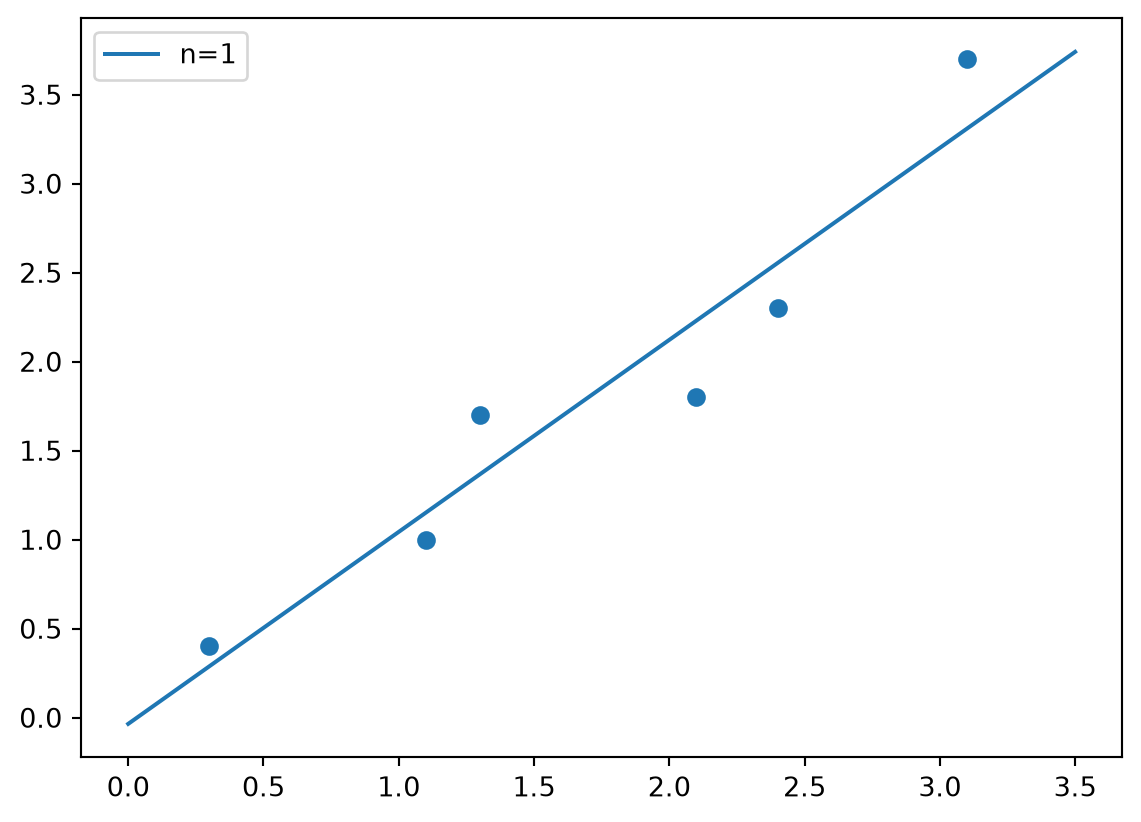
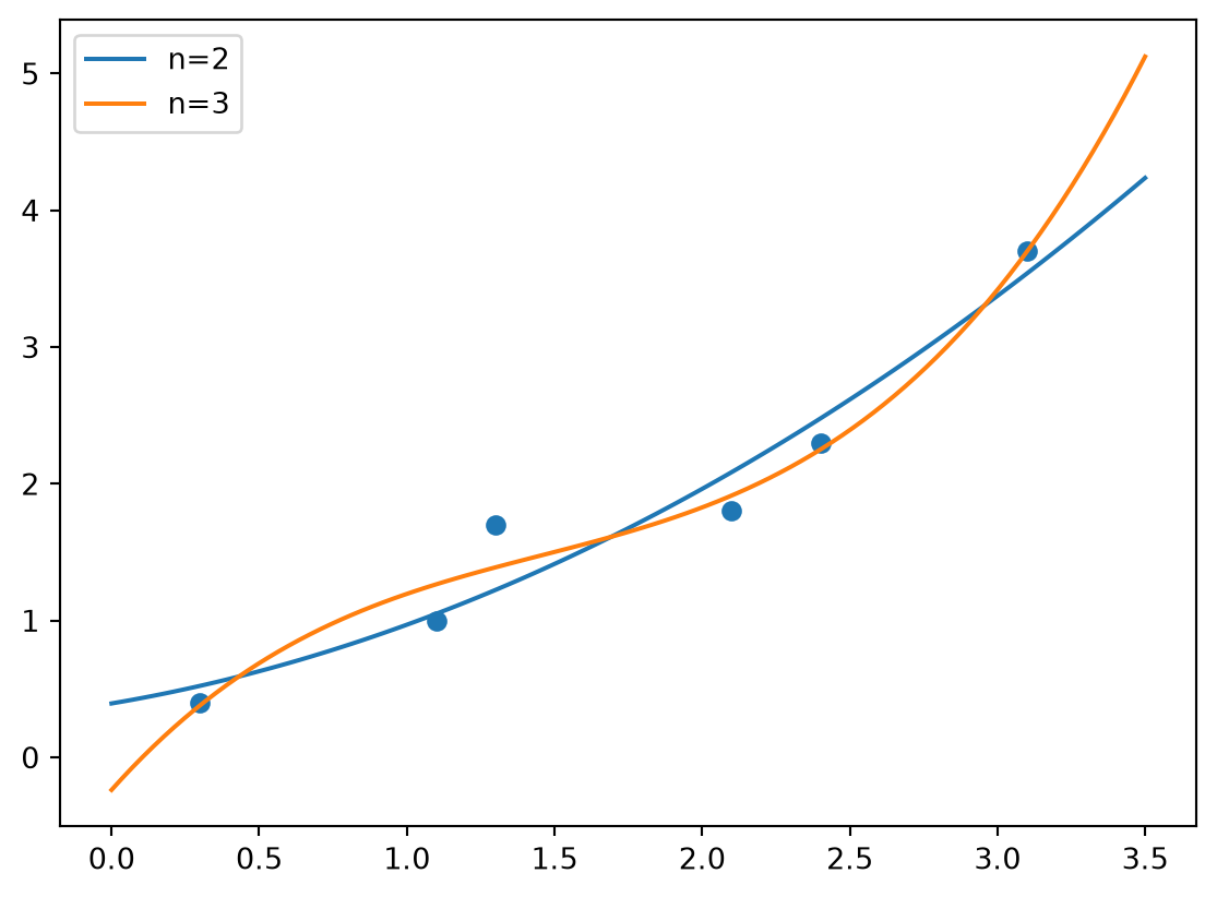
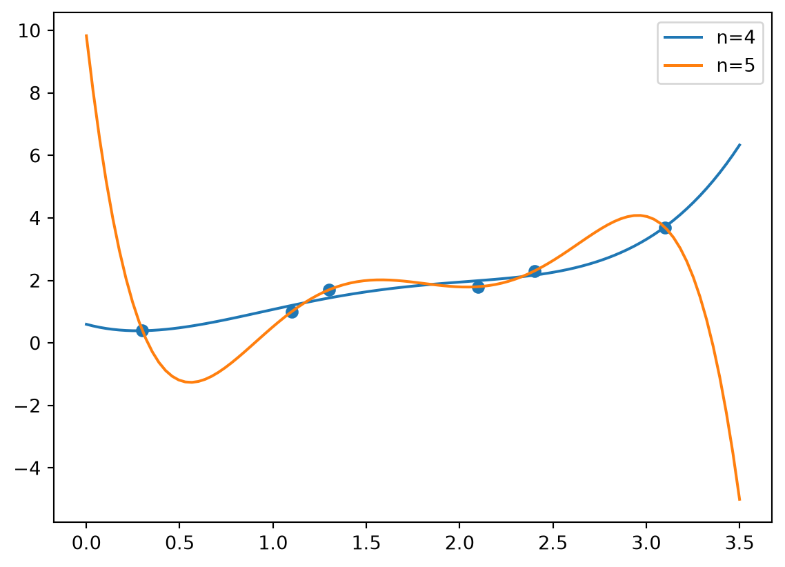
The \(x_i\) here are distinct, so that the least squares solution is unique. In Figure 13.1 least squares fits for higher degree polynomials are shown. The last fit is with a fifth degree polynomial. All fits use 6 points. Since there is a unique polynomial of degree \(5\) passing through these points, it is clear that this fit actually interpolates in the given points (the sum of squared errors is 0). The fourth degree polynomial does not, although it is very close at the given points.
13.4 The Gram-Schmidt process
Proposition 5.5 stated that all subspaces have an orthogonal basis. The proof was unconstructive - no procedure was stated that produced an orthogonal set. Let us remedy this. We start by writing the subspace as a span, \(\text{Sp}(\mathbf{a}_1,...,\mathbf{a}_n)\), where all vectors are linearly independent. Suppose we have found \(r\) vectors \(\mathbf{q}_1,...,\mathbf{q}_r\) which are orthogonal, and so that \[\text{Sp}(\mathbf{q}_1,...,\mathbf{q}_r)=\text{Sp}(\mathbf{a}_1,...,\mathbf{a}_r).\] Now, define \[ \mathbf{q}_{r+1}=\mathbf{a}_{r+1}-\sum_{i=1}^r \frac{ \mathbf{a}_{r+1}\cdot \mathbf{q}_i }{ \mathbf{q}_i\cdot \mathbf{q}_i }\mathbf{q}_i. \tag{13.5}\] For \(1\leq j\leq r\) we have that \[\begin{align*} \mathbf{q}_{r+1}\cdot \mathbf{q}_j &= \mathbf{a}_{r+1}\cdot \mathbf{q}_j - \sum_{i=1}^r \frac{ \mathbf{a}_{r+1}\cdot \mathbf{q}_i }{ \mathbf{q}_i\cdot \mathbf{q}_i }\mathbf{q}_i\cdot \mathbf{q}_j \\ &= \mathbf{a}_{r+1}\cdot \mathbf{q}_j - \frac{ \mathbf{a}_{r+1}\cdot \mathbf{q}_j }{ \mathbf{q}_j\cdot \mathbf{q}_j }\mathbf{q}_j\cdot \mathbf{q}_j \\ &= \mathbf{a}_{r+1}\cdot \mathbf{q}_j - \mathbf{a}_{r+1}\cdot \mathbf{q}_j = 0 \end{align*}\] It follows that \(\mathbf{q}_1,...,\mathbf{q}_{r+1}\) also are orthogonal, and it is easy to see that these have the same span as \(\mathbf{a}_1,...,\mathbf{a}_{r+1}\). We have thus produced an orthogonal basis for \(\text{Sp}(\mathbf{a}_1,...,\mathbf{a}_n)\). The method we have just described for this is also called the Gram-Schmidt process.
13.5 The QR-factorisation
Let \(A\) be an invertible \(n\times n\)-matrix. By a QR-factorisation we mean a factorisation \(A=QR\) so that \(Q\) is orthogonal and \(R\) is upper triangular. It turns out that the Gram-Schmidt process can be used to obtain a QR factorisation of \(A\). To see why, note first that the columns of \(A\), denoted \(\mathbf{a}_i\), are linearly independent, since \(A\) is invertible. This means that we can apply the Gram-Schmidt process to arrive at a set \(\{\mathbf{q}_i\}_{i=1}^n\) of orthogonal vectors. We continue by showing that \[ \begin{pmatrix}\mathbf{a}_1 & \mathbf{a}_2 & \cdots & \mathbf{a}_n \end{pmatrix} = \begin{pmatrix}\mathbf{q}_1 & \mathbf{q}_2 & \cdots & \mathbf{q}_n \end{pmatrix} \begin{pmatrix} 1 & \frac{ \mathbf{a}_2\cdot \mathbf{q}_1 }{ \mathbf{q}_1\cdot \mathbf{q}_1 } & \cdots & \frac{ \mathbf{a}_n\cdot \mathbf{q}_1 }{ \mathbf{q}_1\cdot \mathbf{q}_1 } \\ 0 & 1 & \cdots & \frac{ \mathbf{a}_n\cdot \mathbf{q}_2 }{ \mathbf{q}_2\cdot \mathbf{q}_2 } \\ \vdots & \vdots & \ddots & \vdots \\ 0 & 0 & \cdots & 1 \end{pmatrix} \tag{13.6}\] Start by rewriting Equation 13.5 to \[\begin{align*} \mathbf{a}_{r+1}&=\sum_{i=1}^r \frac{ \mathbf{a}_{r+1}\cdot \mathbf{q}_i }{ \mathbf{q}_i\cdot \mathbf{q}_i }\mathbf{q}_i + \mathbf{q}_{r+1} \\ &= \begin{pmatrix} \mathbf{q}_1 & \mathbf{q}_2 & \cdots & \mathbf{q}_r & \mathbf{q}_{r+1} \end{pmatrix} \begin{pmatrix} \frac{ \mathbf{a}_{r+1}\cdot \mathbf{q}_1 }{ \mathbf{q}_1\cdot \mathbf{q}_1 } \\ \frac{ \mathbf{a}_{r+1}\cdot \mathbf{q}_2 }{ \mathbf{q}_2\cdot \mathbf{q}_2 } \\ \vdots \\ \frac{ \mathbf{a}_{r+1}\cdot \mathbf{q}_r }{ \mathbf{q}_r\cdot \mathbf{q}_r } \\ 1 \end{pmatrix} \\ &= \begin{pmatrix} \mathbf{q}_1 & \mathbf{q}_2 & \cdots & \mathbf{q}_r & \mathbf{q}_{r+1} & \mathbf{q}_{r+2} & \cdots & \mathbf{q}_n \end{pmatrix} \begin{pmatrix} \frac{ \mathbf{a}_{r+1}\cdot \mathbf{q}_1 }{ \mathbf{q}_1\cdot \mathbf{q}_1 } \\ \frac{ \mathbf{a}_{r+1}\cdot \mathbf{q}_2 }{ \mathbf{q}_2\cdot \mathbf{q}_2 } \\ \vdots \\ \frac{ \mathbf{a}_{r+1}\cdot \mathbf{q}_r }{ \mathbf{q}_r\cdot \mathbf{q}_r } \\ 1 \\ 0 \\ \vdots \\ 0 \end{pmatrix}. \end{align*}\] This shows that column \(r+1\) in the left and right hand sides in Equation 13.6 coincide. All columns are therefore equal, so that Equation 13.6 holds.
So far \(Q\) has orthogonal columns. We need also secure that they have unit length. This is easily achieved by rewriting Equation 13.6 to \[ \begin{pmatrix}\mathbf{a}_1 & \mathbf{a}_2 & \cdots & \mathbf{a}_n \end{pmatrix} = \begin{pmatrix}\frac{\mathbf{q}_1}{|\mathbf{q}_1|} & \frac{\mathbf{q}_2}{|\mathbf{q}_2|} & \cdots & \frac{\mathbf{q}_n}{|\mathbf{q}_n|} \end{pmatrix} \begin{pmatrix} |\mathbf{q}_1| & \frac{ \mathbf{a}_2\cdot \mathbf{q}_1 }{ |\mathbf{q}_1| } & \cdots & \frac{ \mathbf{a}_n\cdot \mathbf{q}_1 }{ |\mathbf{q}_1| } \\ 0 & |\mathbf{q}_2| & \cdots & \frac{ \mathbf{a}_n\cdot \mathbf{q}_2 }{ |\mathbf{q}_2| } \\ \vdots & \vdots & \ddots & \vdots \\ 0 & 0 & \cdots & |\mathbf{q}_n| \end{pmatrix} \tag{13.7}\]
The following code computes the two matrices on the right hand sides of Equation 13.7. \(A\) is here the matrix with columns \(\mathbf{a}_i\).
def qrfact(A):
    m, n = np.shape(A)
    Q = np.zeros((m,n)); Q[:,0] = A[:,0];
    R = np.eye(n);
    for j in range(1,n):
        R[[j-1],j:] = (Q[:,[j-1]].T @ A[:,j:])/(Q[:,[j-1]].T @ Q[:,[j-1]])
        Q[:,[j]] = A[:,[j]] - Q[:,:j]@R[:j,[j]]
    norms = np.linalg.norm(Q,axis=0)
    Q = Q@np.diag(1/norms)
    R = np.diag(norms)@R
    return Q, R
Before the for-loop we fill in the first row in the two matrices.
Inside the for-loop the first line fills in row \(j\) in the upper triangular matrix \(R\). To see why, note first that the expression
Q[:,[j-1]].T @ A[:,j:]computes the row vector \[ \begin{pmatrix} \mathbf{a}_{j+1}\cdot \mathbf{q}_{j} & \mathbf{a}_{j+2}\cdot \mathbf{q}_{j} & \cdots & \mathbf{a}_n\cdot \mathbf{q}_{j} \end{pmatrix} \] Similarly, the expression
Q[:,[j-1]].T @ Q[:,[j-1]]computes \(\mathbf{q}_j\cdot \mathbf{q}_j\). These are divided, so that this first line fills out row \(j\) of the upper triangular matrix \(R\) to the right of the diagonal with the values \[ \begin{pmatrix} \frac{\mathbf{a}_{j+1}\cdot \mathbf{q}_j}{\mathbf{q}_j\cdot \mathbf{q}_j} & \frac{\mathbf{a}_{j+2}\cdot \mathbf{q}_j}{\mathbf{q}_{j-1}\cdot \mathbf{q}_j} & \cdots & \frac{\mathbf{a}_n\cdot \mathbf{q}_j}{\mathbf{q}_j\cdot \mathbf{q}_j} \end{pmatrix} \]
After this we have in column \(j\) in \(R\) all coefficients in Equation 13.5, so that we can compute \(\mathbf{q}_{j+1}\). This is done in the second line of the for-loop. Here
Q[:,:j]@R[:j,[j]]simply computes \(\sum_{k=1}^j \frac{\mathbf{a}_j\cdot\mathbf{q}_k}{\mathbf{q}_k\cdot\mathbf{q}_k}\mathbf{q}_k\), so that the second line actually implements Equation 13.5. The result is filled into column \(j+1\) in the matrix \(Q\).
The last lines in qrfact ensure that the columns of \(Q\) have unit length. The call to np.linalg.norm returns a vector comprised of the lengths of the column vectors of \(A\). The columns of \(Q\) are then normalised by multiplying to the right with a diagonal matrix with these lengths on the diagonal. The matrix \(R\) is multiplied with a diagonal matrix to the left instead, so that the net effect of multiplying with these two diagonal matrices is no change. The effect is that we have the QR-factorisation.
Let us test the code on a random \(3\times 3\)-matrix:
A = np.random.rand(3,3)
Q, R = qrfact(A)
A-Q@R
array([[ 0.00000000e+00, 0.00000000e+00, 0.00000000e+00],
[-2.77555756e-17, 0.00000000e+00, 0.00000000e+00],
[ 0.00000000e+00, 0.00000000e+00, 0.00000000e+00]])Let us also test that the \(Q\)-matrix is orthogonal:
Q.T@Qarray([[ 1.00000000e+00, 3.62066974e-16, -3.55122192e-17],
[ 3.62066974e-16, 1.00000000e+00, -4.49460452e-16],
[-3.55122192e-17, -4.49460452e-16, 1.00000000e+00]])13.6 General vector spaces and inner product spaces
Let \(V\) be a set which has two binary operations:
- An operation \(V\times V\to V\), denoted by \(+\) (called vector addition).
- An operation \(V\times\mathbb{C}\to V\) (called scalar multiplication)
\(V\) is called a vector space if the following are satisfied for these operations, any \(\mathbf{u},\mathbf{v},\mathbf{w}\in V\), and any scalars \(s,t\):
- \(\mathbf{u} + (\mathbf{v} + \mathbf{w})=(\mathbf{u} + \mathbf{v}) + \mathbf{w}\) (associativity)
- \(\mathbf{u} + \mathbf{v} = \mathbf{v} + \mathbf{u}\) (Commutativity)
- There exists an element \(\mathbf{0}\in V\) so that \(\mathbf{v}+\mathbf{0}=\mathbf{v}\) for all \(\mathbf{v}\in V\) (\(V\) has an identity)
- For each element \(\mathbf{v}\in V\) there exists an element \(-\mathbf{v}\in V\) so that \(\mathbf{v}+(-\mathbf{v})=\mathbf{0}\).
- \(s(t\mathbf{v})=(st)\mathbf{v}\) (scalars can be moved out)
- \(1\mathbf{v}=\mathbf{v}\) (\(1\in\mathbb{C})\) is a multiplicative identity on \(V\))
- \(s(\mathbf{u}+\mathbf{v})=s\mathbf{u}+s\mathbf{v}\) (vector addition is distributive)
- \((s+t)\mathbf{u} = s\mathbf{u} + t\mathbf{v}\) (scalar addition is distributive)
Any subspace of \(\mathbb{R}^m\) is clearly a vector space. We will also use functions to define new vector spaces. The functions may be restricted to continuous functions or integrable functions. If \(f\) and \(g\) are functions, \(f+g\) is defined as the function defined by \((f+g)(t)=f(t)+g(t)\) for all \(t\). Also, If \(s\) is a scalar, \(sf\) is defined as the function defined by \((sf)(t)=sf(t)\) for all \(t\).
\(V\) is called an inner product space if it is a vector space, and also has an operation \(V\times V\to\mathbf{C}\), (denoted \(\langle\cdot,\cdot\rangle\), and called an inner product), which satisfies, for any \(\mathbf{u},\mathbf{v},\mathbf{w}\in V\) and scalars \(s\) and \(t\)
- \(\langle\mathbf{u},\mathbf{u}\rangle\geq 0\), with equality if and only if \(\mathbf{v}=\mathbf{0}\) (positivity)
- \(\langle\mathbf{u},\mathbf{v}\rangle=\overline{\langle\mathbf{v},\mathbf{u}\rangle}\). (conjugate symmetry)
- \(\langle \mathbf{u}+\mathbf{v},\mathbf{w}\rangle= \langle \mathbf{u},\mathbf{w}\rangle+\langle \mathbf{v},\mathbf{w}\rangle\) and \(\langle \mathbf{u},\mathbf{v}+\mathbf{w}\rangle= \langle \mathbf{u},\mathbf{v}\rangle+\langle \mathbf{u},\mathbf{w}\rangle\) (bi-linearity).
- \(\langle a\mathbf{u},\mathbf{v}\rangle=a\langle \mathbf{u},\mathbf{v}\rangle\) (scalars can be moved out)
The scalar product is in particular an inner product, and which turns any subspace of \(\mathbb{R}^m\) into an inner product space.
Linear independence, span, and bases, are defined for vector spaces as for subspaces of \(\mathbb{R}^m\). We will restrict ourselves to vector spaces that have a finite basis. As before we can show that all basse have the same number of elements, so that it again gives meaning to define the dimension of a (finite-dimensional) vector space.
The coordinate mapping \(\mathbf{x}\to[\mathbf{x}]_{\mathcal{A}}\) is defined as before. Proposition 5.10 stated that, for subspaces of \(\mathbb{R}^m\), this is an isomorphism. The same is the case for finite-dimensional vector spaces, and as previously, the concepts of linear independence, span, and bases can be viewed in terms of the coordinate mapping.
We will also consider function spaces as inner product spaces. Several function spaces will be of interest - polynomials, trigonometric functions, or more generally continuous functions and integrable functions. We will first consider the vector space consisting of polynomials of degree \(\leq n\), \[ \mathcal{P}_n = \text{Span}(1,t,...,t^n), \] which has the basis \(\mathcal{B}=\{1,t,...,t^n\}\).
13.6.1 Discrete inner products on polynomials
Let \(f,g\in\mathcal{P}_n\), and let \(\{x_i\}_{i=1}^m\) be \(m\) distinct points in \(\mathbb{R}\). We will consider \[ \langle f,g \rangle = \sum_{i=1}^m f(x_i)\overline{g(x_i)} \tag{13.8}\] as a candidate for an inner product on \(\mathcal{P}_n\). We have the following result.
Proposition 13.4 Equation 13.8 is an inner product on \(\mathcal{P}_n\) if and only if \(m>n\).
Proof. The only inner product property that may be problematic is whether \(\langle f,f \rangle=0\) implies that \(f=0\). That \(\langle f,f \rangle=0\) is equivalent to \(f(x_1)=f(x_2)=\cdots=f(x_m)=0\). Let us see when such a nonzero \(f\) can be found.
If \(m>n\), \(f\) is a polynomial of degree at most \(n\) with \(m>n\) zeros. But then \(f\) must be identically zero.
If \(m\leq n\), \(f\) is a polynomial of degree at most \(n\) with \(m\leq n\) zeros (at the \(x_i\)). Clearly such a nonzero polynomial exists, so that the positivity part is not fulfilled for all \(f\).
Therefore, Equation 13.8 gives an inner product on \(\mathcal{P}_{m-1},\mathcal{P}_{m-2},...\). The distance associated with this inner product \[\|f-g\|=\sqrt{\sum_{i=1}^m |f(x_i)-g(x_i)|^2}. \tag{13.9}\] We recognise this as the sum of squared errors between \(f\) and \(g\) from Section 13.3. A function \(g\in\mathcal{B}\) minimising this is thus a least square fit to \(f\). it is also the nearest point to \(f\) from \(\mathcal{B}\) in the norm given by Equation 13.9.
Example 13.1 Apply to \(V_{N,T}\). It is also straightforward to show that \[\langle f,g \rangle = \int_0^T f(t)\overline{g(t)}\,dt. \tag{13.10}\] defines an inner product. The associated distance is now \[\|f-g\|=\sqrt{\int_0^T |f(x)-g(x)|^2\,dt}. \tag{13.11}\] This is also called the mean squared error of \(f\) and \(g\) (MSE). In the next section we will consider the nearest point to \(f\) in the norm given by Equation 13.11 when the space in question is a space of trigonometric functions. We will obtain a nice expression for the nearest point in this case since this space has a natural orthogonal basis.
13.7 Orthogonal polynomials
The Gram-Schmidt process can be generalised to inner product spaces by replacing the scalar product with the inner product: \[ \mathbf{q}_{r+1}=\mathbf{a}_{r+1}-\sum_{i=1}^r \frac{ \langle\mathbf{a}_{r+1},\mathbf{q}_i\rangle }{ \langle \mathbf{q}_i,\mathbf{q}_i\rangle }\mathbf{q}_i. \tag{13.12}\] When applying the Gram-Schmidt process in \(\mathbb{R}^m\) the vectors \(\mathbf{a}_i\) are different from the standard basis vectors (the canonical basis), since these are already orthogonal. In general inner product spaces, however, a canonical set of vectors is typically not orthogonal, so that it is natural to apply Gram-Schmidt to these. When looking at polynomials we will thus set \(\mathbf{a}_k=t^{k-1}\), and let \(\mathcal{B}=\{\mathbf{a}_i\}_{i=1}^n\). We will also set \(A=\begin{pmatrix} \mathbf{a}_1 & \mathbf{a}_2 & \cdots & \mathbf{a}_n \end{pmatrix}\). This is new notation for us, since \(A\) is a row vectors where the entries are polynomials. We start by applying the coordinate mapping of \(\mathcal{B}\) (see Section 5.2) on each side in Equation 13.12: \[ [\mathbf{q}_{r+1}]_{\mathcal{B}}=\mathbf{e}_{r+1}-\sum_{i=1}^r \frac{ \langle\mathbf{a}_{r+1},\mathbf{q}_i\rangle }{ \langle \mathbf{q}_i,\mathbf{q}_i\rangle }[\mathbf{q}_i]_{\mathcal{B}}. \] Let us also rewrite the inner products. Using the same coordinate mapping we write \(\mathbf{q}_i = A [\mathbf{q}_i]_{\mathcal B}\) and \[ \begin{aligned} \langle \mathbf{a}_{r+1},\mathbf{q}_i\rangle &= \langle \mathbf{a}_{r+1},A [\mathbf{q}_i]_{\mathcal{B}}\rangle = \sum_l \langle \mathbf{a}_{r+1}, \mathbf{a}_l ([\mathbf{q}_i]_{\mathcal{B}})_l\rangle \\ &= \sum_l \langle \mathbf{a}_{r+1},\mathbf{a}_l\rangle ([\mathbf{q}_i]_{\mathcal{B}})_l = \mathbf{e}_{r+1}^T G [\mathbf{q}_i]_{\mathcal{B}} \\ \langle \mathbf{q}_i,\mathbf{q}_i\rangle &= \langle A [\mathbf{q}_i]_{\mathcal{B}},A [\mathbf{q}_i]_{\mathcal{B}}\rangle = \sum_{k,l} \langle \mathbf{a}_k ([\mathbf{q}_i]_{\mathcal{B}})_k , \mathbf{a}_l ([\mathbf{q}_i]_{\mathcal{B}})_l\rangle \\ &= \sum_{k,l} ([\mathbf{q}_i]_{\mathcal{B}})_k \langle \mathbf{a}_k,\mathbf{a}_l\rangle ([\mathbf{q}_i]_{\mathcal{B}})_l = [\mathbf{q}_i]_{\mathcal B}^T G [\mathbf{q}_i]_{\mathcal{B}} \end{aligned} \] where \(G\) is the matrix with entries \(\langle \mathbf{a}_k,\mathbf{a}_l\rangle\), \(1\leq k,l\leq n\). Equation 13.12 can thus be written \[ [\mathbf{q}_{r+1}]_{\mathcal{B}} =\mathbf{e}_{r+1}-\sum_{i=1}^r \frac{ \mathbf{e}_{r+1}^T G [\mathbf{q}_i]_{\mathcal{B}} }{ [\mathbf{q}_i]_{\mathcal B}^T G [\mathbf{q}_i]_{\mathcal{B}} }[\mathbf{q}_i]_{\mathcal{B}}, \] where now all parts are in euclidean space. The matrix \(G\) is pre-computed. We will look at several examples of this.
Example 13.2 (Discrete Chebyshev polynomials) Let us consider the case where the polynomials are functions defined on \([-1,1]\). We define the inner product as \[\langle f,g\rangle=\frac{1}{m}\sum_{i=1}^m f(x_i)g(x_i)\] where \[ \mathbf{x}=(-1+1/m, -1+2/m,...,1-2/m,1-1/m), \] i.e., \(m\) points spread uniformly on \((-1+1/m,1-1/m)\). Entry \((k,l)\) in \(G\) is \(\frac{1}{m}\sum_{i=1}^m x_i^{k+l-2}\), so that \(G\) can be computed as follows, where we consider the first \(6\) orthogonal polynomials only:
m=6
x = np.linspace(-1+1/m,1-1/m,m)
k = np. arange(1,m+1).reshape((-1,1))
l = np.arange(1,m+1).reshape((1,-1))

G = np.zeros((m,m))
for xval in x:
    G += xval**(k+l-2)
G = G/m
We apply the Gram-Schmidt process and normalise the vectors to have unit length:
R = np.eye(m); A = np.eye(m)
Q = np.zeros((m,m)); Q[:,0] = A[:,0];
for j in range(1,m):
    R[[j-1],j:] = (Q[:,[j-1]].T @ G @ A[:,j:])/(Q[:,[j-1]].T @ G @ Q[:,[j-1]])
    Q[:,[j]] = A[:,[j]] - Q[:,:j]@R[:j,[j]]

for j in range(m):
    nrm = np. sqrt( Q[:,[j]].T @ G @ Q[:,[j]] )
    Q[:,[j]] = Q[:,[j]]/nrm
    R[[j],:] = nrm*R[[j],:]
Then we plot the 6 polynomials together, together with the points in \(\mathbf{x}\).
t = np.linspace(-1,1,100).reshape((-1,1))
p = np.arange(0,m).reshape((1,-1))
The result can be seen in Figure 13.2.
plt.plot( t, t**p @ Q[:,[0]])
plt.plot( t, t**p @ Q[:,[1]])
plt.plot( t, t**p @ Q[:,[2]])
plt.legend(['n=0','n=1','n=2'])
plt.scatter(x,np.zeros(np.shape(x)[0]))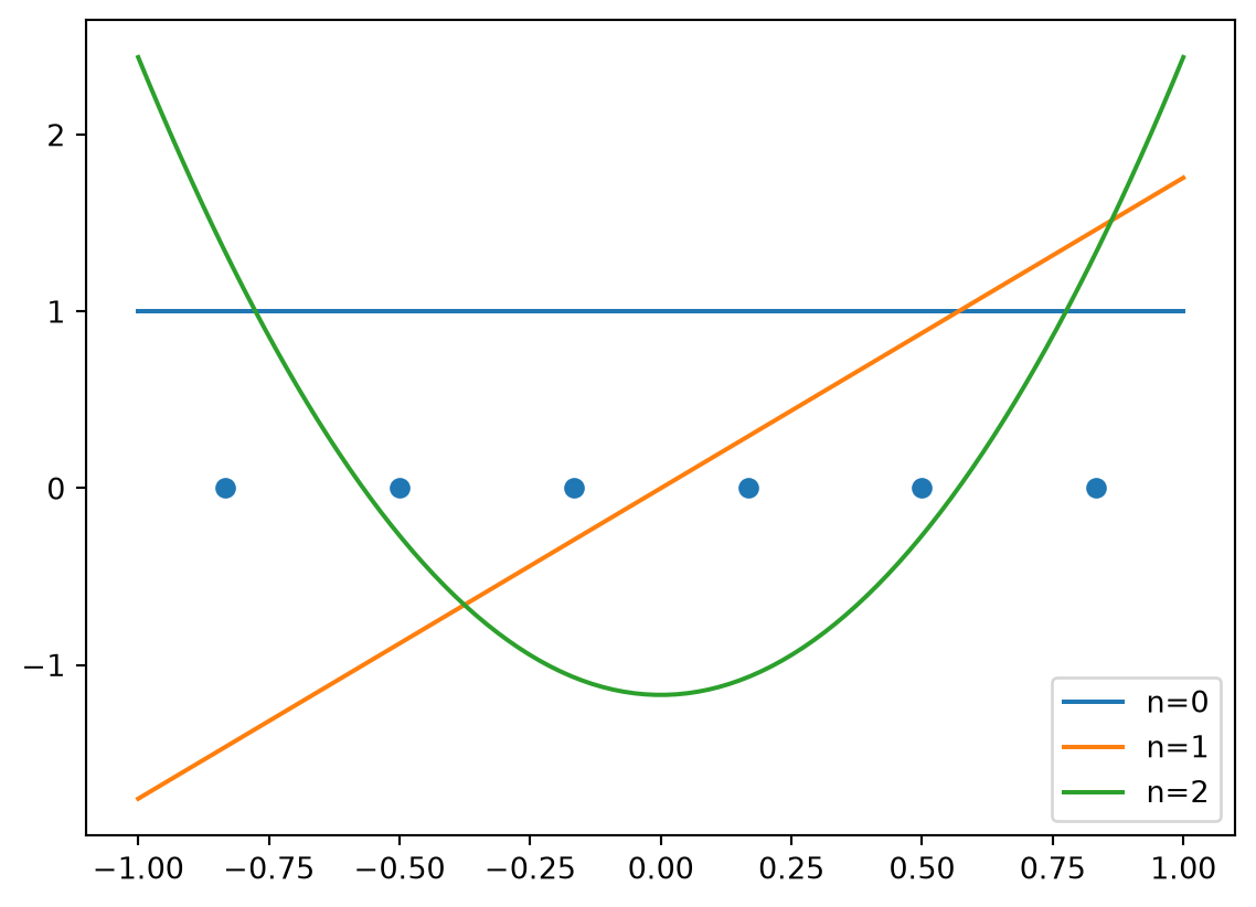
plt.plot( t, t**p @ Q[:,[3]])
plt.plot( t, t**p @ Q[:,[4]])
plt.plot( t, t**p @ Q[:,[5]])
plt.legend(['n=4','n=5','n=6'])
plt.scatter(x,np.zeros(np.shape(x)[0]))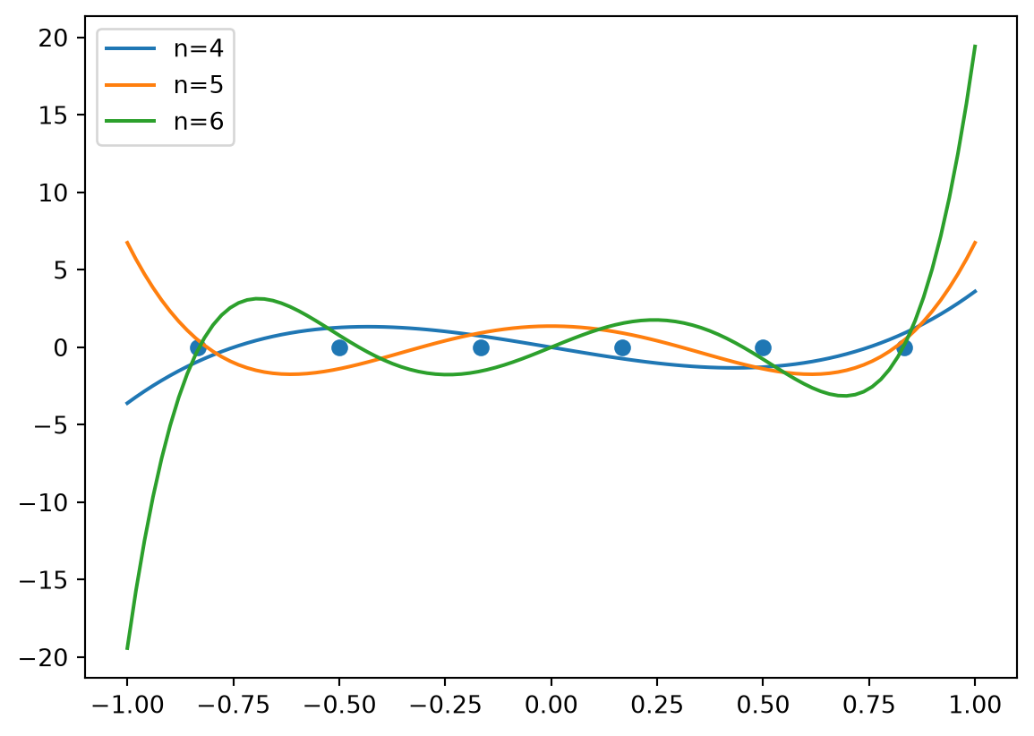
Look at the case where \(G\) is obtained from the inner product is \(\int_a^b t^{k+l-2}w(t)\,dt\).
13.8 Fourier series
In Chapter 10 we produced approximations to a function from the vector space \[V_{N,T}=\text{Span}\{e^{2\pi int/T} \}_{n=-N}^N,\] using interpolation. Let us now instead equip \(V_{N,T}\) with one of the previous inner products, and find the closest point in \(V_{N,T}\) to the function. We start by proving the following.
Proposition 13.5 The functions \(\{e^{2\pi int/T}\}_{n=-N}^N\) are orthogonal w.r.t. the inner product from Equation 13.10.
Proof. We compute \[ \langle e^{2\pi imt/T},e^{2\pi int/T} \rangle = \int_0^T e^{2\pi i(m-n)t/T}\,dt. \] If \(m=n\) this evaluates to \(T\). If \(m\neq n\) we get \[ \frac{T}{2\pi i(m-n)}\left[ e^{2\pi i(m-n)t/T} \right]_0^T = \frac{T}{2\pi i(m-n)} ( e^{2\pi i(m-n)}-e^0 ) = 0, \] since the trigonometric functions have period \(2\pi\). The functions are thus orthogonal.
It follows that \[\begin{align*} \text{proj}_{V_{N,T}}(f) &= \sum_{n=-N}^N \frac{ \langle f,e^{2\pi int/T} \rangle }{ \langle e^{2\pi int/T} , e^{2\pi int/T}\rangle} e^{2\pi int/T} \\ &= \frac{1}{T} \sum_{n=-N}^N \int_0^T f(t)e^{-2\pi int/T}\,dt e^{2\pi int/T} \end{align*}\] This is also called the Fourier series of \(f\). The coefficients of the \(e^{2\pi int/T}\) are called Fourier coefficients. Let us compute the Fourier coefficients of the square wave. When \(n\neq 0\) we get \[\begin{align*} \int_0^T f_s(t)e^{-2\pi int/T}\,dt &= \int_0^{T/2} e^{-2\pi int/T}\,dt - \int_{T/2}^T e^{-2\pi int/T}\,dt \\ &= -\frac{T}{2\pi in}[e^{-2\pi int/T}]_0^{T/2} + \frac{T}{2\pi in}[e^{-2\pi int/T}]_{T/2}^T \\ &= \frac{T}{2\pi in}\left(-e^{-\pi in} + 1 + e^{-2\pi in} - e^{-\pi in}\right) \\ &= \frac{T}{2\pi in} (2-2e^{-\pi in}) = \frac{T}{\pi in} (1-e^{-\pi in}) \\ &= \frac{T}{\pi in} (1-(-1)^n) \end{align*}\] When \(n=0\) we get \(0\). The Fourier series for the square wave is therefore \[ \sum_{-N\leq n\leq N, n\neq 0} \frac{1-(-1)^n}{\pi in} e^{2\pi int/T} \] The following code returns the Fourier coefficients, as well as the corresponding range of \(n\)-values in the sum.
def find_fourier_coeffs(N):
    n = np.arange(-N,N+1).reshape((1,-1)).astype(float)
    n = np.delete(n, N, axis=1)
    c = ((1-(-1)**n)/(np.pi*1j*n)).T
    return c, n
Note that the code discards the value \(n=0\), to avoid division by zero. We can now plot the Fourier series as follows.
def square_wave(t, T):
    return 2*(t < T/2).astype(int) -1

Nvals = [3,7,11]
freq_s = 44100
freq = 440
T= 1/freq
samples_per_period = int(freq_s/freq)
t = np.linspace(0,T,samples_per_period).reshape((-1,1))
plt.plot( t, square_wave(t,T), '-k', label = 'f(t)')

for N in Nvals:
    c, n = find_fourier_coeffs(N)
    p = np.real( np.exp(2*np.pi*1j*n*t/T)@c )
    plt.plot(t, p, label=f"p(t), M={2*N+1}.")
plt.legend()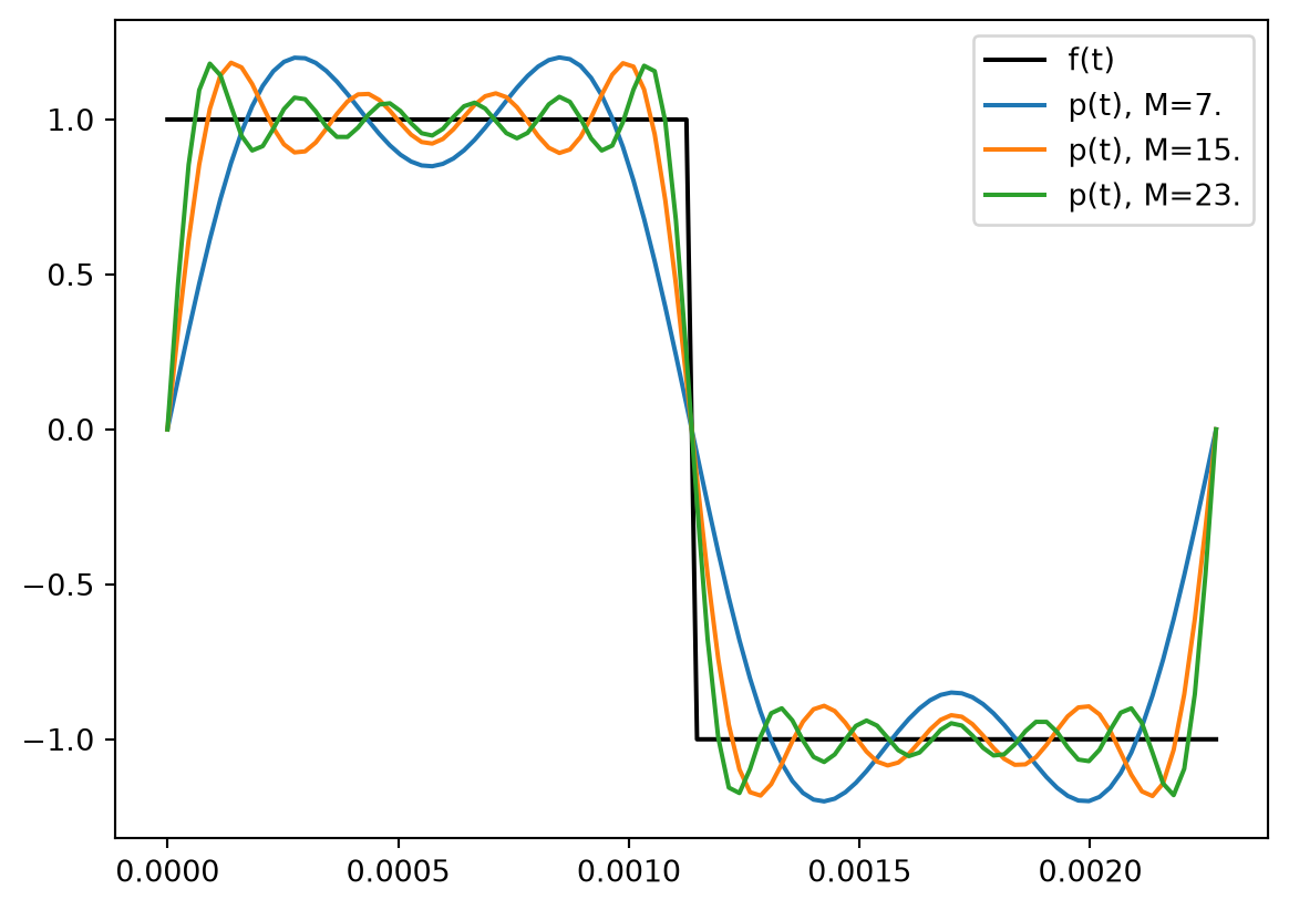
Quiz
Exercises
Exercise 13.1 Apply Gram-Schmidt to a set of vectors
Exercise 13.2 Find a QR-factorisation of a matrix.
Exercise 13.3 The triangle wave was defined in Exercise 10.13 by \[
f_t(t) =
\begin{cases}
\frac{4}{T}\left( \frac{T}{4}-t \right) & \text{ for } 0\leq t<T/2 \\
\frac{4}{T}\left( t - \frac{3T}{4} \right)
\end{cases}
\] It turns out that it is rather tedious to compute the Fourier coefficients of the triangle wave by hand, and symbolic software packages like sympy may not give a nice answer either. Instead we will here attempt to find the Fourier coefficients with a computer program.
- Prove the relations \[\begin{align*} \int_0^{T/2} e^{-2\pi int/T}\,dt &= \frac{T}{2\pi in} (1-(-1)^n) \\ \int_{T/2}^T e^{-2\pi int/T}\,dt &= \frac{T}{2\pi in} ((-1)^n-1) \\ \int_0^{T/2} te^{-2\pi int/T}\,dt &= -\frac{T^2}{4\pi in}(-1)^n + \frac{T}{2\pi in}\int_0^{T/2} e^{-2\pi int/T}\,dt \\ \int_{T/2}^T te^{-2\pi int/T}\,dt &= (-1)^n \left( \frac{T}{2} \int_0^{T/2} e^{-2\pi int/T}\,dt + \int_0^{T/2} te^{-2\pi int/T}\,dt \right) \\ \int_0^{T/2} \frac{4}{T}(T/4-t)e^{-2\pi int/T} \,dt &= \int_0^{T/2} e^{-2\pi int/T}\,dt - \frac{4}{T}\int_0^{T/2} te^{-2\pi int/T}\,dt \\ \int_{T/2}^T \frac{4}{T}(t-3T/4)e^{-2\pi int/T}\,dt &= \frac{4}{T} \int_{T/2}^T te^{-2\pi int/T} - 3\int_{T/2}^T e^{-2\pi int/T}\,dt \\ \int_0^T f_t(t)e^{-2\pi int/T}\,dt &= \int_0^{T/2} \frac{4}{T}(T/4-t)e^{-2\pi int/T} \,dt + \int_{T/2}^T \frac{4}{T}(t-3T/4)e^{-2\pi int/T}\,dt \end{align*}\]
- Write a function
find_fourier_triangle(n)which returns the Fourier coefficients for the triangle wave for the values of \(n\) listed in the vectorn.
- Repeat the setup from Exercise 10.13 in order to plot different Fourier series for the triangle wave.