A=np.array([[1,2,3,4],[2,1,2,3],[3,2,1,2],[4,3,2,1]])
t = np.linspace(-4,10,100).reshape((-1,1))
V = t**(np.arange(4,-1,-1).reshape((1,-1)))
vals = V @ np.poly(A).reshape((-1,1))
plt.plot( t.reshape(-1), vals.reshape(-1) )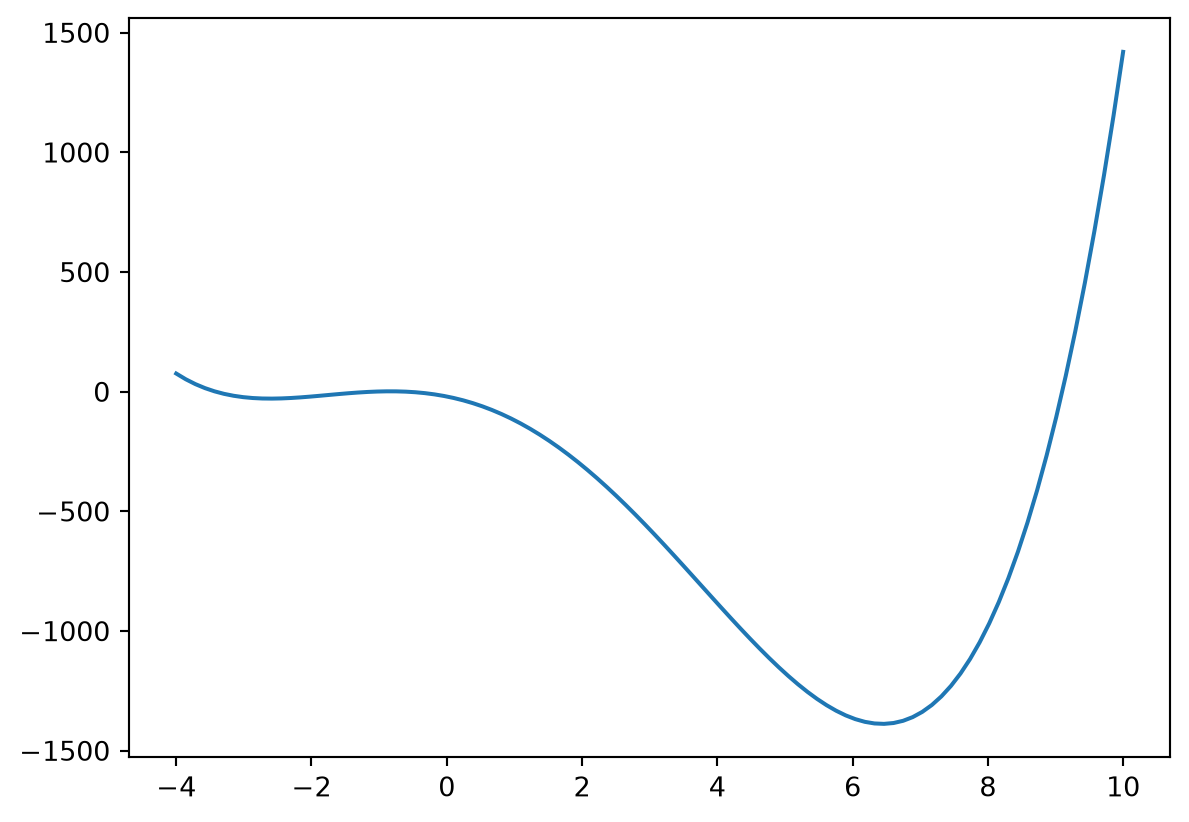
Eigenvectors and eigenvalues are core mathematical objects with many applications. Usually we can’t find them symbolically, however, so that we must rely on numerical methods. Many such methods exist, some of which find both eigenvalues and eigenvectors. Others may only find the eigenvalues, or perhaps only one particular eigenvalue, such as the biggest or smallest one. In this chapter we will encounter some of these methods.
One obvious way to find eigenvalues of a matrix would be to plot the characteristic polynomial, and zoom in to find its zeros. Let us test this approach on the \(4\times 4\)-matrix \(A=\left(\begin{array}{cccc} 1 & 2 & 3 & 4 \\ 2 & 1 & 2 & 3 \\ 3 & 2 & 1 & 2 \\ 4 & 3 & 2 & 1 \end{array} \right)\),
where we start by plotting the characteristic polynomial of \(A\) over \([-4,10]\) (the second line).
A=np.array([[1,2,3,4],[2,1,2,3],[3,2,1,2],[4,3,2,1]])
t = np.linspace(-4,10,100).reshape((-1,1))
V = t**(np.arange(4,-1,-1).reshape((1,-1)))
vals = V @ np.poly(A).reshape((-1,1))
plt.plot( t.reshape(-1), vals.reshape(-1) )
We see that there is a zero in \([8,10]\), so that we can restrict the plot to this interval. The next plot reveals that a zero can be found in the interval \([8.75,9.25]\). Continuing in this way you will find a zero close to \(9.09\).
This method clearly has its limitations. First of all, it has to be repeated for all the other zeros as well. Secondly, for large matrices we encounter polynomials of very high degree, so that the plot values easily become very large.
We start with the Jacobi method, which can be used to find all eigenvectors and eigenvalues of a symmetric matrix numerically. It does so by constructing orthogonal matrices \(P_1,P_2,...\), and successively applying similarity transformations \[ \begin{aligned} A_1 &= A \\ A_2 &= P_1^TA_1P_1 \\ A_3 &= P_2^TA_2P_2 \\ \vdots & \vdots \\ A_{k+1} &= P_k^TA_kP_k \end{aligned} \tag{15.1}\] We first note that all these matrices are symmetric: Set \(B=P^TAP\) with \(A\) symmetric and \(P\) orthogonal. We compute \[B^T=(P^TAP)^T=P^TA^T(P^T)^T=P^TAP=B,\] so that \(B\) also is symmetric.
We also note that all matrices \(A_i\) have the same eigenvalues. To see why, if \(\textbf{v}\) is an eigenvector for \(A_k\) with eigenvalue \(\lambda\), then the last equation above gives \[A_{k+1}(P_k)^T\textbf{v}=(P_k)^TA_k\textbf{v}=\lambda (P_k)^T\textbf{v},\] so that \((P_k)^T\textbf{v}\) is an eigenvector for \(A_{k+1}\), also with eigenvalue \(\lambda\). Since \(A_k\) and \(A_{k+1}\) have the same eigenvalues, all of the \(A_k\) have the same eigenvalues. If \(\textbf{v}\) is an eigenvector of \(A_1=A\), then in particular \((P_1)^T\textbf{v}\) will be an eigenvector of \(A_2\). By repeating this procedure \((P_2)^T(P_1)^T\textbf{v}\) will be an eigenvector for \(A_3\), and more generally \[ (P_k)^T\cdots(P_1)^T\textbf{v} = (P_1\cdots P_k)^T\textbf{v} \] will be an eigenvector for \(A_{k+1}\). Thus, if \(P\) is a matrix consisting of orthonormal eigenvectors for \(A\) (so that \(A=PDP^T\)), \((P_1\cdots P_k)^TP\) is a matrix consisting of orthonormal eigenvectors of \(A_{k+1}\). It follows that \(A_{k+1}=(P_1\cdots P_k)^TPDP^T(P_1\cdots P_k)\), so that \[ A=PDP^T=(P_1\cdots P_k)A_{k+1}(P_1\cdots P_k)^T \] The idea is now to choose the \(P_i\) so that the matrices \(A_i\) get closer to zero outside the diagonal. We will later see that we can achieve this. In other words, if \(A_k=D_k+E_k\), where \(D_k\) is the diagonal part of \(A_k\), and \(E_k\) its off-diagonal part, we can achieve that \(E_k\to 0\). It follows that \((P_1\cdots P_k)D_{k+1}(P_1\cdots P_k)^T\to A\), and by continuity of the eigenvalues that the diagonal elements in \(D_k\) converge to the eigenvalues of \(A\). We will not go into similar arguments for the convergence of \(P_1\cdots P_k\) to a matrix with eigenvectors as columns.
After each transformation \(A_{k+1} = P_k^TA_kP_k\) we will therefore compute \[\text{off}(A) = \sqrt{\sum_{i\neq j}^n a_{ij}^2},\] and if this value is less than a given tolerance, \(A\) is considered ‘diagonal enough’, and the algorithm terminates.
The matrices \(P_k\) will have the following form: \[ P_k = \begin{pmatrix} 1 & 0 & \cdots & \cdots & \cdots & \cdots & \cdots & 0 & 0 \\ 0 & 1 & \cdots & \cdots & \cdots & \cdots & \cdots & \cdots & \cdots \\ \cdots & \cdots & \cdots & \cdots & \cdots & \cdots & \cdots & \cdots & \cdots \\ \cdots & \cdots & \cdots & \cos\theta & \cdots & \sin\theta & \cdots & \cdots & \cdots \\ \cdots & \cdots & \cdots & \cdots & \cdots & \cdots & \cdots & \cdots & \cdots \\ \cdots & \cdots & \cdots & -\sin\theta & \cdots & \cos\theta & \cdots & \cdots & \cdots \\ \cdots & \cdots & \cdots & \cdots & \cdots & \cdots & \cdots & \cdots & \cdots \\ 0 & 0 & \cdots & \cdots & \cdots & \cdots & \cdots & 0 & 1 \end{pmatrix} \tag{15.2}\] where \((P_k)_{rr} = (P_k)_{ss} = \cos\theta\), \((P_k)_{rs} = -(P_k)_{sr} = \sin\theta\), \((P_k)_{ii} = 1\) (for \(i\neq r,s\)) and \(0\) else. \(P_k\) is orthogonal with \[ (P_k)^{-1} = (P_k)^T = \begin{pmatrix} 1 & 0 & \cdots & \cdots & \cdots & \cdots & \cdots & 0 & 0 \\ 0 & 1 & \cdots & \cdots & \cdots & \cdots & \cdots & \cdots & \cdots \\ \cdots & \cdots & \cdots & \cdots & \cdots & \cdots & \cdots & \cdots & \cdots \\ \cdots & \cdots & \cdots & \cos\theta & \cdots & -\sin\theta & \cdots & \cdots & \cdots \\ \cdots & \cdots & \cdots & \cdots & \cdots & \cdots & \cdots & \cdots & \cdots \\ \cdots & \cdots & \cdots & \sin\theta & \cdots & \cos\theta & \cdots & \cdots & \cdots \\ \cdots & \cdots & \cdots & \cdots & \cdots & \cdots & \cdots & \cdots & \cdots \\ 0 & 0 & \cdots & \cdots & \cdots & \cdots & \cdots & 0 & 1 \end{pmatrix} \tag{15.3}\] To see this, let \(C\) be the product of the matrices given by Equation 15.2 and Equation 15.3. Since the rows/columns coincide with the rows/columns of the identity matrix outside row/column \(r\) and \(s\), it is clear that \(c_{kl}=I_{kl}\) when \(k\neq r,s\), \(l\neq r,s\) (\(I\) is the identity matrix). If \(k\neq r,s\) we also see that \(c_{kr}=c_{rk}=c_{ks}=c_{sk}=0\), since columns \(r,s\) are the only ones which have elements in row \(r\) and \(s\). Further we see that \[\begin{eqnarray*} c_{rs} &=& -\cos\theta\sin\theta + \sin\theta\cos\theta = 0\\ c_{sr} &=& -\sin\theta\cos\theta + \cos\theta\sin\theta = 0\\ c_{rr} &=& \cos\theta\cos\theta + \sin\theta\sin\theta = 1\\ c_{ss} &=& (-\sin\theta)(-\sin\theta) + \cos\theta\cos\theta = 1. \end{eqnarray*}\] It is therefore clear that \(C=I\), so that the two matrices are inverses of one-another.
If \(n=2\) the matrix \(P\) corresponds to a rotation with angle \(\theta\) in the plane. The \(P_k\) therefore have inherited the name rotation matrices, since they can be viewed as a rotation when we limit ourselves to the plane spanned by two variables \(x_r\) and \(x_s\), while all other variables are kept fixed.
Let us go through the steps needed to implement Jacobi’s method. The function below takes the position \((r,s)\), the angle \(\theta\), and the dimension \(n\) as arguments, and returns the matrix \(P_k\) in Equation 15.2.
def P_k(r,s,theta,n):
    P = np.eye(n)
    P[r-1,r-1] = np.cos(theta); P[r-1,s-1] = np.sin(theta)
    P[s-1,r-1] = -np.sin(theta); P[s-1,s-1] = np.cos(theta)
    return P
The next functions take a real \(n\times n\)-matrix \(A\) as input. The first returns \(\text{off}(A)\):
def off(A):
    all = np.sum(np.sum(A**2))
    diag = np.sum(np.diag(A)**2)
    return np.sqrt( all - diag )
The next returns the position \((r,s)\) of the element outside the diagonal with biggest absolute value. The np.max-function is used:
def offabsmaks(A):
    B = abs(A)
    n = np.shape(A)[0]
    for k in range(n):
        B[k,k] = 0
    maxvals = np.max(B, axis=0)
    s = np.argmax(maxvals)
    r = np.argmax(B[:, s])
    return r + 1, s + 1
The quantity \(\sqrt{\sum_{i,j} a_{ij}^2}\) is called the Frobenius norm of \(A\), and is written \(\|A\|_F\). We will have use for the fact that, if \(P\) is orthogonal and \(B=PA\), \(A\) and \(B\) have the same Frobenius norm. We say that the Frobenius norm is invariant under orthogonal transformations. Since \((PA)_{:,i}=PA_{:,i}\), it is enough to show this invariance when \(A\) and \(B\) are column vectors. Since the Frobenius norm equals the euclidean norm for column vectors we get \[ | P\mathbf{a}|^2 = (P\mathbf{a})^TP\mathbf{a}=\mathbf{a}^TP^TP\mathbf{a}=\mathbf{a}^T\mathbf{a} =|\mathbf{a}|^2. \] The same can be shown when \(A\) is multiplied with an orthogonal matrix to the left.
By restricting \(B=P^TAP\) to row/columns \(r\) and \(s\), and using that \(A\) and \(B\) have the same Frobenius norm, we get that \[a_{rr}^2 + a_{rs}^2 + a_{sr}^2 + a_{ss}^2 = b_{rr}^2 + b_{rs}^2 + b_{sr}^2 + b_{ss}^2,\] which can also be written as \[a_{rr}^2 + a_{ss}^2 - b_{rr}^2 - b_{ss}^2=2b_{rs}^1-2a_{rs}^2. \tag{15.4}\]
We need to compute the components in the matrix \(P\). Applying the definition of matrix multiplication, and using that \(P\) has nonzero elements only in position \(r\) and \(s\) in row/column \(r\) and \(s\), it is clear that
From the first point above it follows that \(\sum_{i\neq r,s} a_{ii}^2 = \sum_{i\neq r,s} b_{ii}^2\). Adding \(a_{rr}^2+a_{ss}^2+b_{rr}^2+b_{ss}^2\) to both sides gives \[\sum_{i=1}^n a_{ii}^2 + b_{rr}^2 + b_{ss}^2 = \sum_{i=1}^n b_{ii}^2 + a_{rr}^2 + a_{ss}^2,\] which can be written as \[\|A\|_F^2 - \text{off}(A)^2 + b_{rr}^2 + b_{ss}^2 = \|B\|_F^2 - \text{off}(B)^2 + a_{rr}^2 + a_{ss}^2.\] Since \(\|A\|_F=\|B\|_F\) this can be written as \[ \text{off}(B)^2 = \text{off}(A)^2 + a_{rr}^2 + a_{ss}^2 - b_{rr}^2 - b_{ss}^2 = \text{off}(A)^2 + 2b_{rs}^1 - 2a_{rs}^2,\] where we used Equation 15.4. Thus, the off-diagonal contribution \(\text{off}(B)\) only changes due to the \((r,s)\) and \((s,r)\) components, and is smallest when \(r,s\) are chosen so that \(|a_{rs}|\) is as big as possible, and when \(\theta\) is chosen so that \(b_{rs}=0\), The new value is then \(\text{off}(B)^2 = \text{off}(A)^2 - 2a_{rs}^2\).
We have that \(b_{rs}=0\) when \[\sin\theta\cos\theta (a_{rr}-a_{ss}) + (\cos^2\theta-\sin^2\theta)a_{rs} = 0\] This can be rewritten to \(\frac{1}{2}\sin(2\theta)(a_{rr}-a_{ss}) + \cos(2\theta) a_{rs} = 0\), which also can be written \[\tan(2\theta)=\frac{2a_{rs}}{a_{ss}-a_{rr}}. \tag{15.5}\]
Since there are \(n(n-1)\) off-diagonal entries, each of which are less than \(|a_{rs}|\) in absolute value, we have that \(\text{off}(A)^2 \leq n(n-1)a_{rs}^2\). From this it follows that \(-2a_{rs}^2\leq - \frac{2}{n(n-1)}\text{off}(A)^2\), so that \[ \text{off}(B)^2 = \text{off}(A)^2 - 2a_{rs}^2 \leq \text{off}(A)^2 - \frac{2}{n(n-1)}\text{off}(A)^2 = \left(1- \frac{2}{n(n-1)}\right)\text{off}(A)^2. \] From this it follows that the off-diagonal contribution converges to zero, and we argued that this guaranteed convergence to the actual eigenvalues in Jacobi’s method.
The following function returns an approximation to the eigenvalues and the eigenvectors of a given matrix with help of Jacobi’s method.
def eig_jacobi(A):
    tol=10**(-4)
    n = np.shape(A)[0]
    P = np.eye(n)
    while off(A) > tol:
        r, s = offabsmaks(A)
        theta = np.arctan( 2*A[r-1,s-1]/(A[s-1,s-1]-A[r-1,r-1]) )/2
        Pk = P_k(r, s, theta, n)
        A = Pk.T @ A @ Pk
        P = P @ Pk
    return A, P
Inside the loop \(r,s\) are first found as the off-diagonal entry with largest absolute value, \(\theta\) is found from Equation 15.5, and the matrix \(P_k\) is computed. The variable A is updated to \(A_2\), \(A_3\), and so on, while the variable P is updated to \(P_1\), \(P_1P_2\), \(P_1P_2P_3\), and so on. The code stops when \(\text{off}(A_k)\) gets smaller than the given tolerance. To test this we create a random \(6\times 6\) matrix \(A\). \(A+A^T\) is then a symmetric matrix:
A = np.random.rand(6,6)
A = A+A.T
Our method gives the following approximation to the eigenvalues:
D, P = eig_jacobi(A)
np.diag(D)
array([-0.22185337, 5.66061091, -1.5386142 , 1.29258601, 0.21695214,
0.87443915])We first verify that the columns in \(P\) are eigenvectors. This is the same as testing that \(PDP^T\) is an orthogonal diagonalisation of \(A\):
A - P @ D @ P.Tarray([[ 6.66133815e-16, 6.66133815e-16, 2.22044605e-16,
4.99600361e-16, 2.22044605e-16, 6.66133815e-16],
[ 4.44089210e-16, 2.22044605e-16, 0.00000000e+00,
5.55111512e-16, 2.22044605e-16, 0.00000000e+00],
[ 5.55111512e-16, 6.66133815e-16, -3.19189120e-16,
4.44089210e-16, 1.11022302e-16, 2.22044605e-16],
[ 5.55111512e-16, 5.55111512e-16, 3.33066907e-16,
6.66133815e-16, 3.33066907e-16, 6.66133815e-16],
[ 1.11022302e-16, 1.11022302e-16, -5.55111512e-17,
3.05311332e-16, 2.22044605e-16, 0.00000000e+00],
[ 2.22044605e-16, 4.44089210e-16, 1.11022302e-16,
6.66133815e-16, 2.22044605e-16, -4.44089210e-16]])It is seen that \(A-PDP^T\) is not exactly zero, but very close to zero. This is due to roundoff errors on the computer. We then test that we get the same eigenvalues as returned by np.linalg.eig:
D, P = np.linalg.eig(A)
D
array([ 5.66061091, -1.5386142 , -0.22185337, 0.21695214, 1.29258601,
0.87443915])We see that eig_jacobi and np.linalg.eig give approximately the same values, but they are listed in a different order. On a computer we have no control over the order eigenvalues are listed - the algorithm decides this along the way.
The matrix \(A\) may be very large, and the function \(P_k\) allocates a matrix of the same size. The following function implements multiplication with \(P_k\) to the right, and avoids this problem simply by re-computing columns \(r\) and \(s\) (these are the only two columns in \(A\) and \(AP_k\) which differ).
def mult_Pk_right(A, r, s, theta):
    a = np.cos(theta)*A[:,[r-1]] - np.sin(theta)*A[:,[s-1]]
    b = np.sin(theta)*A[:,[r-1]] + np.cos(theta)*A[:,[s-1]]
A[:,[r-1,s-1]] = np.block([[a,b]])The QR-method is a method for finding eigenvalues which is very similar to Jacobi’s method. Again we start with a symmetric matrix \(A\), and apply similarity transformations as in the setup in Equation 15.1 (so that all matrices have the same eigenvalues), In Jacobi’s method the similarity transformations were plane rotations, but in the QR-method they are given by the QR-factorisation: If \(A_k=Q_kR_k\) is a QR-factorisation of \(A_k\), we set \(A_{k+1}=Q_k^TA_kQ_k\). We now get \(A_{k+1}=Q_k^TQ_kR_kQ^k=R_kQ_k\). We can test this code on the same matrix \(A\) as before, with small modifications to eig_jacobi above:
def eig_qr(A):
    tol=10**(-4)
    n = np.shape(A)[0]
    P = np.eye(n)
    while off(A) > tol:
        Q, R = np.linalg.qr(A)
        A = R @ Q
        P = P @ Q
    return A, P
The function np.linalg.qr() to used to find the \(QR\) factorisation here.
D, P = eig_qr(A)
np.diag(D)
array([ 5.66061091, -1.5386142 , 1.29258601, 0.87443915, -0.22185336,
0.21695213])A - P @ D @ P.Tarray([[-1.55431223e-15, 2.22044605e-16, -1.22124533e-15,
6.10622664e-16, -1.27675648e-15, -1.11022302e-15],
[ 2.22044605e-16, 1.11022302e-16, -5.55111512e-15,
-4.44089210e-16, -7.77156117e-16, -2.88657986e-15],
[-8.88178420e-16, -6.43929354e-15, 3.09474668e-15,
-3.44169138e-15, -9.99200722e-16, 1.66533454e-15],
[ 4.44089210e-16, -7.77156117e-16, -2.88657986e-15,
-3.55271368e-15, -1.94289029e-16, -1.11022302e-16],
[-9.43689571e-16, -8.88178420e-16, -1.22124533e-15,
2.77555756e-17, -3.21964677e-15, -1.77635684e-15],
[-1.11022302e-15, -2.22044605e-15, 1.33226763e-15,
-1.11022302e-16, -1.55431223e-15, -1.99840144e-15]])D, P = np.linalg.eig(A)
Darray([ 5.66061091, -1.5386142 , -0.22185337, 0.21695214, 1.29258601,
0.87443915])We will not prove that the QR-method converges towards the eigenvalues/eigenvectors.
As we have noted, finding roots in polynomials (i.e., eigenvalues) can be difficult It turns out that this problem can be turned around: We can use linear algebra to find the roots of the characteristic polynomial. In fact, most software find eigenvalues using this approach, rather than finding them directly as roots in a polynomial!
Given the polynomial \[ p(t)=a_0+a_1t+\cdots + a_{n-1}t^{n-1}+t^n,\] we define the companion matrix \(C(p)\) by \[ C(p) = \left(\begin{array}{rrrrr} 0 & 1 & 0 & \cdots & 0 \\ 0 & 0 & 1 & \cdots & 0 \\ \vdots & \vdots & \vdots & \vdots & \vdots \\ 0 & 0 & 0 & \cdots & 1 \\ -a_0 & -a_1 & -a_2 & \cdots & -a_{n-1} \end{array}\right). \]
Let us find the characteristic polynomial of \(C(p)\). We have that \[ C(p) - \lambda I = \left(\begin{array}{rrrrr} -\lambda & 1 & 0 & \cdots & 0 \\ 0 & -\lambda & 1 & \cdots & 0 \\ \vdots & \vdots & \vdots & \vdots & \vdots \\ 0 & 0 & 0 & \cdots & 1 \\ -a_0 & -a_1 & -a_2 & \cdots & -a_{n-1} - \lambda I \end{array}\right). \] When expanding the determinant along the last row we get the minors \[1,-\lambda,\lambda^2,...,(-1)^{n-1}\lambda^{n-1},\] so that the determinant is \[\begin{align*} & \sum_{k=1}^{n-1} (-1)^{n+k+1}a_{k-1} (-1)^{k-1}\lambda^{k-1} + (-1)^{2n+1}(a_{n-1}+\lambda) (-1)^{n-1}\lambda^{n-1} \\ &= (-1)^n \sum_{k=1}^{n-1} a_{k-1} \lambda^{k-1} + (-1)^n\lambda^n (a_{n-1}\lambda^{n-1} +\lambda^n) \\ &= (-1)^n \sum_{k=1}^n a_{k-1} \lambda^{k-1} + (-1)^n\lambda^n \\ &= (-1)^n p(\lambda). \end{align*}\] Since \(\det(C(p)-\lambda I)=(-1)^n p(\lambda)\) it follows that the roots of \(p\) are the eigenvalues of \(C(p)\).
A matrix is invertible if and only if \(\lambda=0\) is not an eigenvalue, and \(\lambda=0\) is a root in \((-1)^n p(\lambda)\) if and only if \(a_0=0\). Thus, \(C(p)\) is invertible if and only if \(a_0\neq 0\). We can also verify that \[ \begin{pmatrix} 0 & 1 & 0 & \cdots & 0 \\ 0 & 0 & 1 & \cdots & 0 \\ \vdots & \vdots & \vdots & \vdots & \vdots \\ 0 & 0 & 0 & \cdots & 1 \\ -a_0 & -a_1 & -a_2 & \cdots & -a_{n-1} \end{pmatrix}\ \begin{pmatrix} -\frac{a_1}{a_0} & -\frac{a_2}{a_0} & \cdots & -\frac{a_{n-1}}{a_0} & -\frac{1}{a_0}\\ 1 & 0 & \cdots & 0 & 0 \\ 0 & 1 & \cdots & 0 & 0 \\ \vdots & \vdots & \vdots & \vdots & \vdots \\ 0 & 0 & \cdots & 1 & 0 \end{pmatrix}=I_n\] component by component, so that \[ C(p)^{-1} = \left(\begin{array}{rrrrr} -\frac{a_1}{a_0} & -\frac{a_2}{a_0} & \cdots & -\frac{a_{n-1}}{a_0} & -\frac{1}{a_0}\\ 1 & 0 & \cdots & 0 & 0 \\ 0 & 1 & \cdots & 0 & 0 \\ \vdots & \vdots & \vdots & \vdots & \vdots \\ 0 & 0 & \cdots & 1 & 0 \end{array}\right). \]
Suppose that \(\lambda\) is a root in \(p(t)\), i.e., an eigenvalue for \(C(p)\). We have that \[\begin{align*} &\left(\begin{array}{rrrrr} 0 & 1 & 0 & \cdots & 0 \\ 0 & 0 & 1 & \cdots & 0 \\ \vdots & \vdots & \vdots & \vdots & \vdots \\ 0 & 0 & 0 & \cdots & 1 \\ -a_0 & -a_1 & -a_2 & \cdots & -a_{n-1} \end{array}\right) \begin{pmatrix} 1 \\ \lambda \\ \lambda^2 \\ \vdots \\ \lambda^{n-1} \end{pmatrix} \\ &= \begin{pmatrix} \lambda \\ \lambda^2 \\ \vdots \\ \lambda^{n-1} \\ -a_0-a_1\lambda-a_2\lambda^2 - \cdots - a_{n-1}\lambda^{n-1} \end{pmatrix} = \begin{pmatrix} \lambda \\ \lambda^2 \\ \vdots \\ \lambda^{n-1} \\ \lambda^n-p(\lambda) \end{pmatrix} = \begin{pmatrix} \lambda \\ \lambda^2 \\ \vdots \\ \lambda^{n-1} \\ \lambda^n \end{pmatrix} \\ &= \lambda \begin{pmatrix} 1 \\ \lambda \\ \lambda^2 \\ \vdots \\ \lambda^{n-1} \end{pmatrix} \end{align*}\] Thus, \((1,\lambda,\lambda^2,...,\lambda^{n-1})\) is a corresponding eigenvector for \(C(p)\)
In the following we shall let \(\lambda_1,...,\lambda_n\) be the roots in \(p(t)\), repeated with multiplicity. Define the Vandermonde matrix \[\mathbf{V} = \begin{pmatrix} 1 & 1 & \cdots & 1 \\ \lambda_1 & \lambda_2 & \cdots & \lambda_n \\ \vdots & \vdots & \vdots & \vdots \\ \lambda_1^{n-1} & \lambda_2^{n-1} & \cdots & \lambda_n^{n-1} \end{pmatrix}.\] We have learned that \(V\) is invertible if and only if the \(\lambda_i\) are distinct (i.e., all eigenvalues have multiplicity one). Let \(D\) be the diagonal matrix with \(\lambda_1,...,\lambda_n\) on the diagonal. We then have that \[C(p)=VDV^{-1},\] so that \(C(p)\) is diagonalisable, with \(V\) diagonalising it.
We can also define the companion matrix \(C(A)\) of a matrix \(A\) to be the companion matrix of \((-1)^n\) times the characteristic polynomial of \(A\).
The following function takes a square matrix \(A\) as input, and returns the companion matrix \(C(A)\).
def C(A):
    n=np.shape(A)[0]
    pol=np.poly(A)
    pol=np.flip(pol)      # Reverse the order, since the highest coefficients are first
    C = np.zeros((n,n))
    C[:(n-1),1:] = np.eye(n-1)
    C[n-1,:] = -pol[:n]
    return C
The function np.poly(A) is used to find the characteristic polynomial of \(A\).
\(C(A)\) and \(A\) have the same eigenvalues, since they by definition have the same characteristic polynomial. Aided by Exercise 3, \(C(A)\) can be constructed without actually knowing the eigenvalues. Since \(C(A)\) has a simpler form (most elements in the matrix are \(0\)), it is easier computationally to compute powers of this matrix.
This makes it computationally easier to use the power method (and other methods!), which enables us to find the unknown eigenvalues.
The function power_impl below takes a matrix \(A\) and an integer \(n\) as input, computes \(C(A)\), performs \(n\) iterations of the power method, and returns the corresponding estimate for the biggest eigenvalue. The function sets the vector having \(1\) in all components as initial vector for the power method:
def power_impl(A,k):
    n = np.shape(A)[0]
    x = np.ones((n,1))
    for r in range(k):
        x = A @ x
        mu = np.max(abs(x))
        x = (1/mu)*x
    return mu, x
mu, x = power_impl(C(A),10)
munp.float64(5.660646982266638)D, P = np.linalg.eig(A)
Darray([ 5.66061091, -1.5386142 , -0.22185337, 0.21695214, 1.29258601,
0.87443915])```