def C(A):
    n=np.shape(A)[0]
    pol=np.poly(A)
    pol=np.flip(pol)      # Reverse the order, since the highest coefficients are first
    C = np.zeros((n,n))
    C[:(n-1),1:] = np.eye(n-1)
    C[n-1,:] = -pol[:n]
return C3 Project: The companion matrix
3.1 Introduction
We have learned that we can find the eigenvalues of a matrix by finding the roots of the characteristic polynomial, but finding the roots of a high degree polynomial can be difficult in itself! It turns out that this problem can be turned up side down: We can in fact use linear algebra to find the roots of the characteristic polynomial. In fact, most software find eigenvalues by following this approach, rather than finding them directly as roots in a polynomial! We shall look at this linear algebra procedure, which can be viewed as a general method for finding roots in polynomials numerically. Given the polynomial p(t)=a_0+a_1t+\cdots + a_{n-1}t^{n-1}+t^n, we define the companion matrix C(p) by C(p) = \left(\begin{array}{rrrrr} 0 & 1 & 0 & \cdots & 0 \\ 0 & 0 & 1 & \cdots & 0 \\ \vdots & \vdots & \vdots & \vdots & \vdots \\ 0 & 0 & 0 & \cdots & 1 \\ -a_0 & -a_1 & -a_2 & \cdots & -a_{n-1} \end{array}\right).
Exercise 3.1
- Show that the characteristic polynomial of C(p) is given by \det(C(p)-\lambda I)=(-1)^n p(\lambda), so that the eigenvalues of C(p) correspond to the roots of p.
Expand the determinant along the last row.
ImportantSolution
We have C(p) - \lambda I = \left(\begin{array}{rrrrr} -\lambda & 1 & 0 & \cdots & 0 \\ 0 & -\lambda & 1 & \cdots & 0 \\ \vdots & \vdots & \vdots & \vdots & \vdots \\ 0 & 0 & 0 & \cdots & 1 \\ -a_0 & -a_1 & -a_2 & \cdots & -a_{n-1} - \lambda I \end{array}\right). When expanding the determinant along the last row we get the minors 1,-\lambda,\lambda^2,...,(-1)^{n-1}\lambda^{n-1}, so that the determinant is \begin{align*} \lefteqn{ \sum_{k=1}^{n-1} (-1)^{n+k+1}a_{k-1} (-1)^{k-1}\lambda^{k-1} + (-1)^{2n+1}(a_{n-1}+\lambda) (-1)^{n-1}\lambda^{n-1} } \\ &= (-1)^n \sum_{k=1}^{n-1} a_{k-1} \lambda^{k-1} + (-1)^n\lambda^n (a_{n-1}\lambda^{n-1} +\lambda^n) \\ &= (-1)^n \sum_{k=1}^n a_{k-1} \lambda^{k-1} + (-1)^n\lambda^n \\ &= (-1)^n p(\lambda). \end{align*}
- Show that C(p) is invertible if and only if a_0\neq 0, and that C(p)^{-1} = \left(\begin{array}{rrrrr} -\frac{a_1}{a_0} & -\frac{a_2}{a_0} & \cdots & -\frac{a_{n-1}}{a_0} & -\frac{1}{a_0}\\ 1 & 0 & \cdots & 0 & 0 \\ 0 & 1 & \cdots & 0 & 0 \\ \vdots & \vdots & \vdots & \vdots & \vdots \\ 0 & 0 & \cdots & 1 & 0 \end{array}\right).
ImportantSolution
A matrix is invertible if and only if \lambda=0 is not an eigenvalue, and \lambda=0 is a root in (-1)^n p(\lambda) if and only if a_0=0. For the second part we compute \left(\begin{array}{rrrrr} 0 & 1 & 0 & \cdots & 0 \\ 0 & 0 & 1 & \cdots & 0 \\ \vdots & \vdots & \vdots & \vdots & \vdots \\ 0 & 0 & 0 & \cdots & 1 \\ -a_0 & -a_1 & -a_2 & \cdots & -a_{n-1} \end{array}\right) \left(\begin{array}{rrrrr} -\frac{a_1}{a_0} & -\frac{a_2}{a_0} & \cdots & -\frac{a_{n-1}}{a_0} & -\frac{1}{a_0}\\ 1 & 0 & \cdots & 0 & 0 \\ 0 & 1 & \cdots & 0 & 0 \\ \vdots & \vdots & \vdots & \vdots & \vdots \\ 0 & 0 & \cdots & 1 & 0 \end{array}\right) component by component.
Exercise 3.2 Suppose that \lambda is a root in p(t), in other words an eigenvalue for C(p) according to Exercise 1. Show that (1,\lambda,\lambda^2,...,\lambda^{n-1}) is a corresponding eigenvector for C(p).
ImportantSolution
We have that \begin{align*} \lefteqn{ \left(\begin{array}{rrrrr} 0 & 1 & 0 & \cdots & 0 \\ 0 & 0 & 1 & \cdots & 0 \\ \vdots & \vdots & \vdots & \vdots & \vdots \\ 0 & 0 & 0 & \cdots & 1 \\ -a_0 & -a_1 & -a_2 & \cdots & -a_{n-1} \end{array}\right) \begin{pmatrix} 1 \\ \lambda \\ \lambda^2 \\ \vdots \\ \lambda^{n-1} \end{pmatrix} } \\ &= \begin{pmatrix} \lambda \\ \lambda^2 \\ \vdots \\ \lambda^{n-1} \\ -a_0-a_1\lambda-a_2\lambda^2 - \cdots - a_{n-1}\lambda^{n-1} \end{pmatrix} = \begin{pmatrix} \lambda \\ \lambda^2 \\ \vdots \\ \lambda^{n-1} \\ \lambda^n-p(\lambda) \end{pmatrix} = \begin{pmatrix} \lambda \\ \lambda^2 \\ \vdots \\ \lambda^{n-1} \\ \lambda^n \end{pmatrix} \\ &= \lambda \begin{pmatrix} 1 \\ \lambda \\ \lambda^2 \\ \vdots \\ \lambda^{n-1} \end{pmatrix} \end{align*}
In the following we shall let \lambda_1,...,\lambda_n be the roots in p(t), repeated with multiplicity. Define the Vandermonde matrix \mathbf{V} = \left(\begin{array}{rrrr} 1 & 1 & \cdots & 1 \\ \lambda_1 & \lambda_2 & \cdots & \lambda_n \\ \vdots & \vdots & \vdots & \vdots \\ \lambda_1^{n-1} & \lambda_2^{n-1} & \cdots & \lambda_n^{n-1} \end{array} \right). It is clear that V is not invertible when a \lambda_i has multiplicity larger than 1, since two columns in V then are equal. V is invertible when the \lambda_1,\ldots\lambda_n are distinct, since eigenvectors for distinct eigenvalues are linearly independent - this implies that the columns in V provide a basis. It follows that V is invertible if and only if all \lambda_1,...,\lambda_n are distinct. Let D be the diagonal matrix with \lambda_1,...,\lambda_n on the diagonal. We then have that C(p)=VDV^{-1}, so that C(p) is diagionalisable, with V diagonalising it.
We can also define the companion matrix C(A) of a matrix A to be the companion matrix of (-1)^n times the characteristic polynomial of A.
Exercise 3.3 Write a function which takes a square matrix A as input, and returns the companion matrix C(A). You can use the command in to find the characteristic polynomial of A.
ImportantSolution
The code can look as follows.
C(A) and A have the same eigenvalues, since they by definition have the same characteristic polynomial. Aided by Exercise 3, C(A) can be constructed without actually knowing the eigenvalues. Since C(A) has a simpler form (most elements in the matrix are 0), it is easier computationally to compute powers of this matrix.
This makes it computationally easier to use the power method (and other methods!), which enables us to find the unknown eigenvalues.
Exercise 3.4 Write a function power_impl which takes a matrix A and an integer n as input, computes C(A), performs n iterations of the power method, and returns the corresponding estimate for the biggest eigenvalue. As initial vector for the power method you can choose the vector having 1 in all components.
ImportantSolution
The code can look as follows.
def power_impl(A,k):
    n = np.shape(A)[0]
    x = np.ones((n,1))
    for r in range(k):
        x = A @ x
        mu = np.max(abs(x))
        x = (1/mu)*x
    return mu, x
With the power method we only found approximations to the biggest eigenvalue above. The QR factorization is a method which can be used to find all the eigenvalues, not only the biggest. If A=QR is the QR-factorisation of A, then the matrices QR and RQ are similar (this is Exercise 5.2.31 in @lay), so that they have the same eigenvalues. If we then define A_1=RQ=Q_1R_1 (where Q_1R_1 is the QR-factorisation of A_1), and then A_2=R_1Q_1=Q_2R_2 (where Q_2R_2 is the QR-factorisation of A_2), and so on, we get a sequence of matrices A,A_1,A_2,\ldots, which all have the same eigenvalues.
Exercise 3.5
- Write a function
qr_implwhich prints the matrices A_1, A_2, A_n, following the recipe above (A and n as input again). Use the built-in functionnp.linalg.qr()to find the QR factorisation of a matrix.
ImportantSolution
def qr_impl(A,n):
    Q, R = np.linalg.qr(A)
    for k in range(n):
        A = R @ Q
        Q, R = np.linalg.qr(A)
print(A)- We now define the matrix A=\left(\begin{array}{cccc} 1 & 2 & 3 & 4 \\ 2 & 1 & 2 & 3 \\ 3 & 2 & 1 & 2 \\ 4 & 3 & 2 & 1 \end{array} \right). Plot the characteristic polynomial of A over [-4,10]. Do you find any zeros? Restrict the plot interval gradually so that you can read out more precise approximations to the zeros, and write down these.
ImportantSolution
The following code can be used.
A=np.array([[1,2,3,4],[2,1,2,3],[3,2,1,2],[4,3,2,1]])
t = np.linspace(-4,10,100).reshape((-1,1))
V = t**(np.arange(4,-1,-1).reshape((1,-1)))
vals = V @ np.poly(A).reshape((-1,1))
plt.plot( t.reshape(-1), vals.reshape(-1) )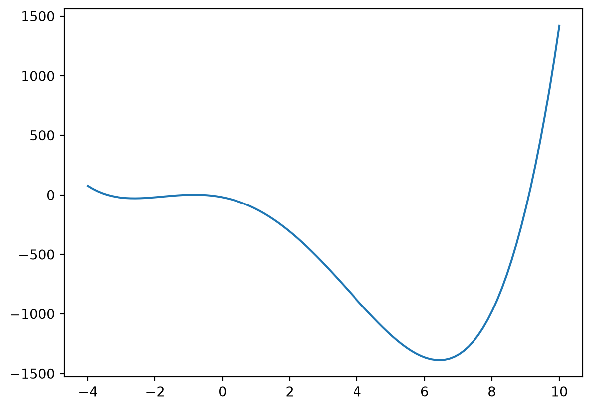
On the second line the plot interval [-4,10] i set. This can be restricted further to for instance [8,10], since the plot shows that there clearly is a zero in this interval. The next plot reveals that a zero can be found in the interval [8.75,9.25]. Continuing in this way you will find a zero close to 9.09. This procedure has to be repeated for te other zeros as well.
- Consider the matrices printed out when running
qr_impl(A,10)[[ 6.93333333 -3.40312648 -3.0568684 1.12687234]
[-3.40312648 -0.64761905 -0.11268723 -0.07529233]
[-3.0568684 -0.11268723 -1.33333333 0.4454354 ]
[ 1.12687234 -0.07529233 0.4454354 -0.95238095]]
[[ 8.75332068 1.95819079 0.59870267 0.09975148]
[ 1.95819079 -2.80787919 -0.67318142 -0.08218431]
[ 0.59870267 -0.67318142 -1.25587673 -0.24165857]
[ 0.09975148 -0.08218431 -0.24165857 -0.68956476]]
[[ 9.04934967e+00 -7.83053713e-01 -7.61037275e-02 6.98176802e-03]
[-7.83053713e-01 -3.33385557e+00 -2.62074284e-01 1.85469051e-02]
[-7.61037275e-02 -2.62074284e-01 -1.09893146e+00 1.24089845e-01]
[ 6.98176802e-03 1.85469051e-02 1.24089845e-01 -6.16562647e-01]]
[[ 9.09200494e+00 2.96040556e-01 9.21147368e-03 4.60136447e-04]
[ 2.96040556e-01 -3.40400729e+00 -8.57805493e-02 -3.33255471e-03]
[ 9.21147368e-03 -8.57805493e-02 -1.09318394e+00 -6.75911170e-02]
[ 4.60136447e-04 -3.33255471e-03 -6.75911170e-02 -5.94813711e-01]]
[[ 9.09803145e+00 -1.11183010e-01 -1.11179824e-03 2.98184348e-05]
[-1.11183010e-01 -3.41289564e+00 -2.76274195e-02 5.77240631e-04]
[-1.11179824e-03 -2.76274195e-02 -1.09675520e+00 3.64031374e-02]
[ 2.98184348e-05 5.77240631e-04 3.64031374e-02 -5.88380605e-01]]
[[ 9.09888039e+00 4.17236920e-02 1.34241006e-04 1.92323076e-06]
[ 4.17236920e-02 -3.41404030e+00 -8.89005005e-03 -9.92605957e-05]
[ 1.34241006e-04 -8.89005005e-03 -1.09831407e+00 -1.94690840e-02]
[ 1.92323076e-06 -9.92605957e-05 -1.94690840e-02 -5.86526018e-01]]
[[ 9.09899993e+00 -1.56561476e-02 -1.62123485e-05 1.23880320e-07]
[-1.56561476e-02 -3.41419044e+00 -2.86120550e-03 1.70401941e-05]
[-1.62123485e-05 -2.86120550e-03 -1.09881272e+00 1.03876473e-02]
[ 1.23880319e-07 1.70401941e-05 1.03876473e-02 -5.85996765e-01]]
[[ 9.09901676e+00 5.87464704e-03 1.95813084e-06 7.97647512e-09]
[ 5.87464704e-03 -3.41421044e+00 -9.20959410e-04 -2.92408696e-06]
[ 1.95813083e-06 -9.20959410e-04 -1.09896011e+00 -5.53831242e-03]
[ 7.97647558e-09 -2.92408696e-06 -5.53831242e-03 -5.85846209e-01]]
[[ 9.09901913e+00 -2.20433689e-03 -2.36509258e-07 5.13540032e-10]
[-2.20433689e-03 -3.41421314e+00 -2.96447745e-04 5.01715462e-07]
[-2.36509259e-07 -2.96447745e-04 -1.09900257e+00 2.95221143e-03]
[ 5.13539558e-10 5.01715462e-07 2.95221143e-03 -5.85803420e-01]]
[[ 9.09901946e+00 8.27130563e-04 2.85665454e-08 3.30611143e-11]
[ 8.27130563e-04 -3.41421350e+00 -9.54247010e-05 -8.60817968e-08]
[ 2.85665441e-08 -9.54247010e-05 -1.09901469e+00 -1.57359020e-03]
[ 3.30615925e-11 -8.60817968e-08 -1.57359020e-03 -5.85791262e-01]]What do you observe? Explain how you now can see approximations to the eigenvalues of A. Are they close to the actual eigenvalues?
ImportantSolution
It looks like the matrices A_n get more and more diagonal, The actual eigenvalues can be found as follows.
D,P = np.linalg.eig(A)
D
array([ 9.09901951, -3.41421356, -1.09901951, -0.58578644])The entries on the diagonal in the A_n seem to be close to this, so that we have obtained good approximations to the eigenvalues.
It is not always the case that the method above gives good approximations to the eigenvalues. We shall not go into when this does, or does not occur.